NER Guide 2026: GLiNER, spaCy, Transformers, and LLMs

Named entity recognition (NER) now spans compact encoders, open-vocabulary models, and LLM-based extraction. In the cited CrossNER evaluation, a 300M-parameter GLiNER model exceeds the reported zero-shot F1 of 13B UniNER. A newer bi-encoder reports up to 130 times the throughput of the comparable gliner_small-v2.5 uni-encoder at 1,024 entity types when labels are pre-computed. The paper measured this on a single H100 with batch size 1 across 64-, 256-, and 512-token inputs. These results motivate experiments, not a universal production ranking.
The companion repository provides runnable examples for GLiNER, ONNX export, LLM-generated training labels, and structured extraction. For workloads dominated by explicit spans, compact encoders are usually the faster and cheaper option. LLMs remain useful for producing training data and handling cases that require inference or normalization.
This guide is for engineers choosing and evaluating NER architectures for RAG, agent, document, or privacy pipelines. You will leave with a model-selection path, a bounded evaluation plan, and a three-tier design for combining encoders with LLM extraction.
Companion repo: ner-field-guide, with runnable demos for GLiNER, ONNX export, the LLM-as-teacher pipeline, and structured extraction with Instructor.
For the short model comparison, see Best NER Models in 2026.
What is named entity recognition?
Named entity recognition finds spans in text and assigns types such as person, organization, date, product, or domain-specific labels. NER identifies the mention. Entity linking is the separate step that resolves a mention to a canonical record or ontology concept.
| Workload | First model to test | Escalate when |
|---|---|---|
| Stable labels and ample training data | spaCy or a fine-tuned encoder | The label set changes or recall stalls on rare types. |
| Changing labels; small type inventory | GLiNER cross-encoder | The inventory grows or labels are reused across many documents. |
| Large, reusable type inventory | GLiNER bi-encoder | The domain set shows a quality or calibration regression. |
| Several extraction tasks in one text pipeline | GLiNER2 | Joint-task quality misses the per-task target. |
| Implicit facts or schema reasoning | Structured LLM extraction | Latency, cost, or unsupported claims exceed the product budget. |
Where modern systems use NER
NER still finds spans of text and assigns labels to them. What changed is its position in the system. It now supplies filters for RAG, structured arguments for agent tools, and fields for document-processing pipelines. Those uses make latency, cost, and schema flexibility as important as benchmark accuracy.
RAG: better retrieval through entity extraction
Similarity search alone struggles when a question contains exact entities. For “what did Anthropic say about model safety in Q4 2024?”, the system should extract “Anthropic” and “Q4 2024” as metadata filters instead of relying only on embeddings.
During indexing, you extract entities from each chunk and store them as metadata: {"organizations": ["Anthropic"], "dates": ["Q4 2024"], ...}. This lets you filter by entity before running vector search. Knowledge graph RAG (GraphRAG, LlamaIndex property graphs) goes further: NER plus relation extraction builds a graph that can answer multi-hop questions that flat embeddings cannot.
At query time, entities extracted from the user’s question drive routing. A question mentioning a company name goes to a finance index; one mentioning drug names goes to a clinical knowledge base. GLiNER is useful when the query-time schema or entity types change. Unseen company or drug names alone do not require open-vocabulary labels; a closed-label model can still recognize new mentions of known types.
AI agents: turning text into structured facts
Agents receive unstructured text such as web pages, API responses, and user messages. NER converts that text into structured facts the agent can reason over, store, or pass to tools.
For tool routing, a request such as “schedule a meeting with Sarah Chen from Accenture on Thursday at 2pm” requires PERSON: Sarah Chen, ORGANIZATION: Accenture, and DATETIME: Thursday 2pm before the agent calls the calendar API. A local encoder avoids the API round trip and is often substantially faster, but latency depends on the model, runtime, hardware, batch size, and label count. Measure both paths on the calendar workload instead of assuming a fixed millisecond gap.
NER also supports entity tracking across conversations. Agent memory systems need to know that “Sarah” in turn 3 and “Ms. Chen” in turn 12 are the same person. NER identifies the spans; entity linking resolves them to the same ID.
The constraint in both cases is latency. If each of ten sequential steps makes a 200 ms NER call, those NER calls add 2 seconds of perceived delay. One call adds 200 ms. Encoder models usually fit entity work inside agent loops better than LLM-based extraction.
Document intelligence: from images to structured data
OCR turns images into text. NER turns that text into structured fields.
A standard pipeline first uses OCR, such as Tesseract, Azure Document Intelligence, or AWS Textract, to produce text and bounding boxes. NER then extracts fields such as invoice_number, vendor_name, line_items, total, and due_date. The same sequence applies to contracts, medical records, and regulatory filings.
Modern document pipelines may combine layout understanding, entity extraction, and relation extraction. OCR or a layout-aware document model still supplies text, reading order, tables, and bounding boxes. GLiNER 2 can then combine entity, relation, classification, and hierarchical structured extraction over that text in one schema-driven pass.
Cost decides most of these pipelines. Price yours at the actual monthly document volume, including retries and review. A compact encoder can run on CPU, while an API-based LLM adds per-document inference cost and latency. A practical test is to label a representative invoice set with an LLM. Fine-tune GLiNER on the reviewed records, then compare both paths on field-level F1, latency, and total cost.
PII detection and LLM guardrails
GDPR’s data-protection principles and security duties (Articles 5, 25, and 32), HIPAA’s technology-neutral Security Rule (HHS guidance), and California’s CCPA as amended by CPRA impose different rights and risk-based safeguards. The cited provisions do not prescribe NER or a specific pre-model scanning architecture. This is not legal advice; have counsel review the requirements that apply to your data and jurisdiction. NER can support data inventory, minimization, or de-identification, but it is one control whose recall must be validated for the relevant data and jurisdiction.
NER handles this directly. De-identification models find PERSON, SSN, PHONE, EMAIL, and ADDRESS spans and either redact them or replace them with synthetic equivalents. Microsoft Presidio combines recognizers with anonymization operators, and its samples include GLiNER as a recognizer. The 0.3B-parameter GLiNER2-PII is another candidate: its paper covers 42 PII types at character-span resolution. Neither is compliance evidence. Validate recall by data format, jurisdiction, language, and PII class before using any detector as a control.
In John Snow Labs’ vendor-run comparison of 48 expert-annotated open-source documents covering six PHI classes, its token-level evaluation reported 96% F1. It reported 91% for Azure, 83% for AWS, and 79% for GPT-4o. The study mapped provider labels to its ground-truth schema and excluded unmappable predictions. Treat it as a narrow provider comparison rather than compliance evidence. A separate deployment report describes Providence processing more than 100,000 clinical notes per day.
For LLM guardrails, NER works as a pre-screening layer: scan user input for PII before sending it to an external API, then block or anonymize. It may be faster or simpler than asking the LLM to self-moderate. Treat that as a deployment hypothesis: measure both paths on your model, hardware, input mix, and recall target. False negatives remain possible, so add another control for the PII exposure your system cannot accept. GLiNER is especially useful here because PII categories vary by jurisdiction. You can add new entity types like “genetic information” under a new regulation without retraining.
GLiNER: span-to-label matching for open-vocabulary NER
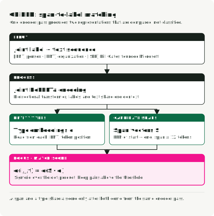
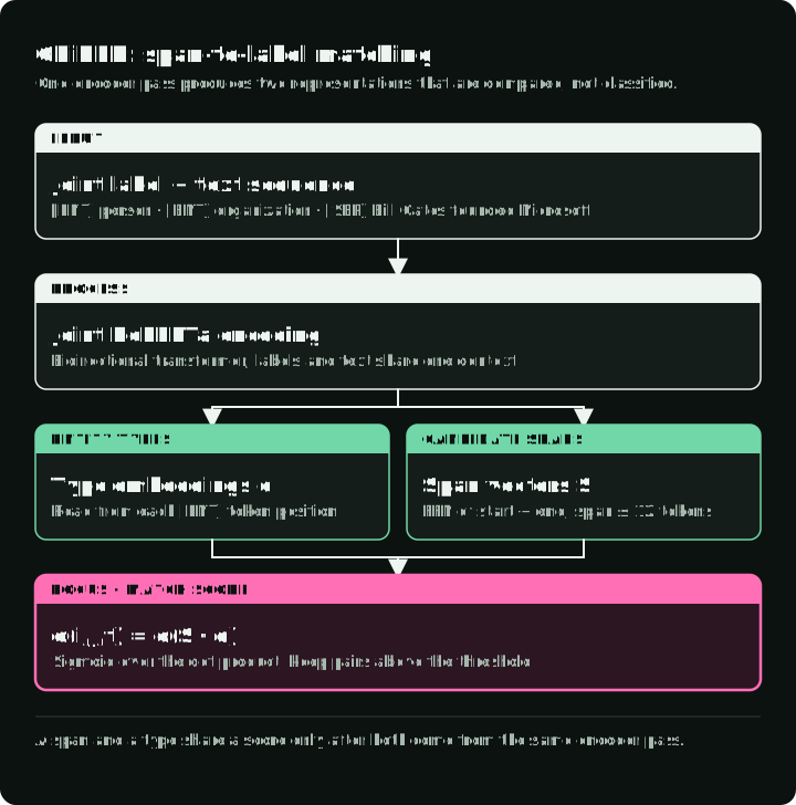
GLiNER (NAACL 2024, Zaratiana et al.) made encoder-based NER competitive with LLMs at a fraction of the cost. Instead of treating NER as sequence labeling or text generation, GLiNER treats it as a matching problem. It scores every candidate text span (each contiguous sequence of words like “Bill Gates” or “Microsoft”) against every entity type label, then keeps the high-scoring pairs.
The model takes entity type labels and input text as a single sequence: [ENT] person [ENT] organization [ENT] date [SEP] Bill Gates founded Microsoft.... A bidirectional transformer (DeBERTa-v3) encodes everything together.
From the output, the model builds two sets of representations. One represents entity types from [ENT] token positions. The other represents text spans by combining start and end token vectors through a small FFN. A dot product between a span representation and an entity type representation gives a score.
Apply sigmoid and you get the probability that the span from token to token belongs to entity type : . Here is the span vector produced by the FFN and is the entity type embedding from the corresponding [ENT] token (Zaratiana et al., 2024, Eqs. 1–2). Spans are capped at 12 tokens to keep things fast.
GLiNER accepts natural-language label descriptions at inference time without retraining, but extraction quality depends on label wording and domain fit. You pass in entity types such as “person,” “adverse drug reaction,” or “financial instrument,” and the model scores spans against them. The 50M, 90M, and 300M configurations below are the original paper models. The current v2.1 model card instead lists 166M, 209M, and 459M English checkpoints, plus a 209M multilingual checkpoint, all under Apache 2.0. Do not compare latency or memory across those generations as if the parameter names were identical (GLiNER v2.1 model card).
For a true hard zero-shot test, hold out target types as well as target examples. A type description such as “a medically confirmed adverse effect caused by a treatment” gives the model more information than adverse event alone. That is not a guarantee of transfer, but description-driven ZeroNER outperformed name-only baselines on its held-out-type benchmarks (Cocchieri et al., 2025).
Training data for the original model came from the Pile-NER dataset: 44,889 passages with 240K entity spans across 13K entity types, all labeled by ChatGPT. Training GLiNER-L took about 5 hours on a single A100 (Zaratiana et al., 2024).
Benchmark results
Zero-shot results from Zaratiana et al. (2024), Tables 1 and 2:
| Model | Params | CrossNER F1 | Avg (20 datasets) |
|---|---|---|---|
| GLiNER-L | 300M | 60.9% | 47.8% |
| GoLLIE | 7B | 58.0% | — |
| UniNER-13B | 13B | 55.6% | — |
| GLiNER-M | 90M | 55.4% | — |
| UniNER-7B | 7B | 53.7% | 45.7% |
| GLiNER-S | 50M | 52.7% | — |
| ChatGPT (GPT-3.5) | — | 47.5% | 36.5% |
GLiNER-M at 90M parameters nearly matches UniNER-13B in the paper’s CrossNER table (55.4% vs. 55.6% F1) while using roughly 140 times fewer parameters. The 50M GLiNER-S exceeds the reported ChatGPT (GPT-3.5) result by 5 F1 points. The multilingual variant, trained only on English data, exceeds that same ChatGPT baseline in 8 of 10 non-English languages (Zaratiana et al., 2024). These comparisons use the paper’s model versions and evaluation harness; they do not establish a ranking against newer LLMs.
GLiNER variants cover biomedical text, PII detection, news, and multilingual support.
From scripts/01_gliner_quickstart.py:
from gliner import GLiNER

model = GLiNER.from_pretrained("urchade/gliner_medium-v2.1")
text = "Bill Gates founded Microsoft on April 4, 1975."
labels = ["person", "organization", "date"]
entities = model.predict_entities(text, labels, threshold=0.5)

for entity in entities:
    print(f"  {entity['text']} => {entity['label']}")
# Bill Gates => person
# Microsoft => organization
# April 4, 1975 => date
How GLiNER compares to spaCy
spaCy is one of the most established NLP libraries in production. It also works under different architectural constraints than GLiNER.
spaCy’s pipelines (en_core_web_sm, en_core_web_trf) do closed-vocabulary NER: a fixed set of entity types (PERSON, ORG, GPE, DATE, etc.) defined at training time. Want a new entity type? Collect labeled data and retrain. Pin the maintained 3.8 model package rather than assuming an unreleased major line is a production upgrade. The en_core_web_trf 3.8.0 model card reports 90.19 NER F1 on OntoNotes 5.0, but only for its 18 predefined types (spaCy model card).
GLiNER does open-vocabulary NER: any label works at inference time, no retraining needed. This makes it the better choice when entity types are unknown in advance, change often, or are domain-specific (“adverse drug reaction”, “financial instrument”, “threat indicator”).
My recommendation: use spaCy for standard entity types where pretrained pipelines are well validated. Use GLiNER when you need flexible, zero-shot types or when your pipeline must adapt without retraining. They can share a pipeline, with spaCy handling tokenization and sentence splitting and GLiNER handling entity extraction.
A supervised Transformer baseline
For stable labels with representative annotated spans, start with a fine-tuned token classifier such as RoBERTa or DeBERTa as the supervised baseline. It trades label flexibility for task-specific accuracy. Compare it with spaCy and GLiNER on exact-span F1, per-label recall, calibration, latency, and cost on the same domain set.
UniNER and NuNER: how small can you go?
UniNER (ICLR 2024, Zhou et al.) and NuNER (EMNLP 2024, Bogdanov et al.) both distill LLM annotations into smaller NER models — but they disagree on how small you can go.
UniNER: the maximalist path
UniNER fine-tunes LLaMA-7B/13B on 45,889 input-output pairs generated by ChatGPT. For each entity type, the model answers “What describes [type] in the text?” and outputs JSON lists. A key training trick: frequency-based negative sampling boosts F1 from 31.5% to 53.4% (Zhou et al., 2024).
UniNER-7B hits 41.7% zero-shot F1 across 43 datasets — beating ChatGPT’s 34.9% by 7 points. The 13B variant reaches 43.4%, only 1.7 points more for nearly double the compute (Zhou et al., 2024).
The production trade-off: the paper’s higher-scoring UniNER-type setup queries each entity type sequentially. Its all-in-one variant uses one response but averaged 3.3% lower. At FP16, a 7B checkpoint needs roughly 14GB just for weights; lower-bit quantization can reduce that footprint. The model also has a restrictive CC BY-NC 4.0 license.
NuNER: the minimalist path
NuNER starts from RoBERTa-base (125M parameters) and uses contrastive training with 4.38 million GPT-3.5 annotations across 200K concepts. After training, the concept encoder is thrown away; the text encoder slots into any standard NER pipeline as a RoBERTa replacement (Bogdanov et al., 2024).
NuNER beats plain RoBERTa by 6-15 F1 points across all few-shot sizes. With just a dozen examples per entity type, NuNER matches UniNER-7B despite being 56x smaller (Bogdanov et al., 2024).
Both papers support distilling LLM annotations into smaller NER models. NuNER shows that a 125M-parameter encoder can match the reported UniNER-7B result when task-specific fine-tuning data is available, with MIT licensing and CPU-friendly inference.
GLiNER 2: one model, four tasks
The original GLiNER ecosystem split NER, relation extraction, classification, and document-level extraction across separate models. The EMNLP 2025 GLiNER2 paper unified NER, classification, and hierarchical extraction in one 205M-parameter model; current releases later added relation extraction to the same schema interface.
The architecture keeps the cross-encoder design but extends context to 2,048 tokens (4x the original) and adds declarative schemas for defining extraction tasks. Training uses 135,698 real documents annotated with GPT-4o plus 118,636 synthetic examples (Zaratiana et al., 2025).
On zero-shot CrossNER, GLiNER 2 scores 0.590 F1, close to GPT-4o’s 0.599 in the paper’s mid-2025 benchmark. For classification, it averages 0.72 across 7 benchmarks, compared with 0.69 for DeBERTa-v3-large. On CPU, the paper reports 130-208 ms classification latency across its tested label counts. The DeBERTa baseline rises from 1,714 ms for 5 labels to 16,897 ms for 50 (Zaratiana et al., 2025).
from gliner2 import GLiNER2
extractor = GLiNER2.from_pretrained("fastino/gliner2-base-v1")

# Multi-task composition in ONE forward pass
schema = (extractor.create_schema()
    .entities({"person": "Names of people", "company": "Organization names"})
    .classification("sentiment", ["positive", "negative", "neutral"])
    .relations(["works_for", "founded", "located_in"])
    .structure("product_info")
        .field("name", dtype="str")
        .field("price", dtype="str"))
text = "Acme launched a $19 widget in Berlin."
results = extractor.extract(text, schema)
Current GLiNER2 releases expose entity recognition, classification, hierarchical extraction, and relation extraction through one schema. The EMNLP paper evaluates NER and classification; it reports no hierarchical-extraction benchmark and does not cover the later relation API. Treat the four-task path as a deployment capability to benchmark, not evidence that one model preserves four specialized models’ accuracy.
2026 additions: choose the architecture that matches the bottleneck
The GLiNER ecosystem now has distinct architectures. They are candidates for a domain comparison, not a single leaderboard.
| Need | Candidate | What to verify |
|---|---|---|
| Many reusable entity types | GLiNER bi-encoder | Exact-span F1 and calibration after caching type embeddings. |
| Entities and relations in one pass | GLiNER-Relex | Both span and relation F1 on the same documents. |
| Local PII candidate | GLiNER2-PII | Recall by language, document format, and PII type. |
| Multilingual open-vocabulary candidate | GLiNER-X | Per-language quality; its card lists 23 languages. |
| Generated or changing types | GLiNER Decoder | Whether generated types are stable and useful downstream. |
The original GLiNER paper, the bi-encoder paper, and GLiNER-Relex each use their own models and harnesses. GLiNER-X and GLiNER Decoder model cards describe released checkpoints, but they are not a peer-reviewed, comparable benchmark. Keep that distinction in an architecture decision record.
Checkpoint licenses are part of the model choice
Verify the exact code, weight, and dataset terms before deployment. The current cited releases are not interchangeable:
| Release | Published license | Practical consequence |
|---|---|---|
| GLiNER v2.1 and GLiNER bi | Apache 2.0 | Permissive model-card terms; still review dependencies and data. |
| GLiNER2 and GLiNER2-PII | Apache 2.0 | Confirm the selected checkpoint, not only the library. |
| UniNER-7B-all | CC BY-NC 4.0 | Do not use for a commercial path without separate permission. |
| NuNER | MIT | The released model and dataset state MIT terms. |
License labels are not legal advice. A production review must include base-model, training-data, and provider terms.
The bi-encoder: scaling to million-label NER
The original GLiNER encodes labels and text together. Joint encoding becomes progressively more expensive as label text consumes the context and must be re-encoded with every document. The crossover depends on the checkpoint, label descriptions, and hardware. When the same large type inventory is reused across many documents, make the GLiNER bi-encoder the default comparison. It splits text and label encoding into two separate transformers (Stepanov et al., 2026).
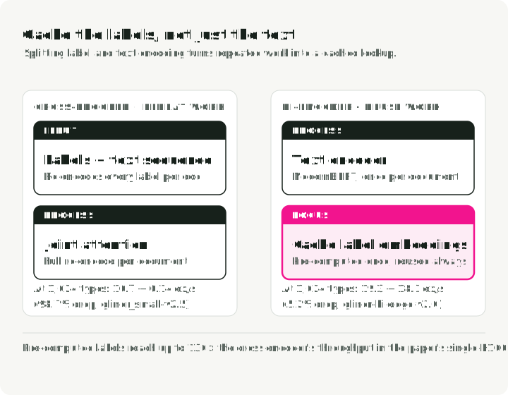
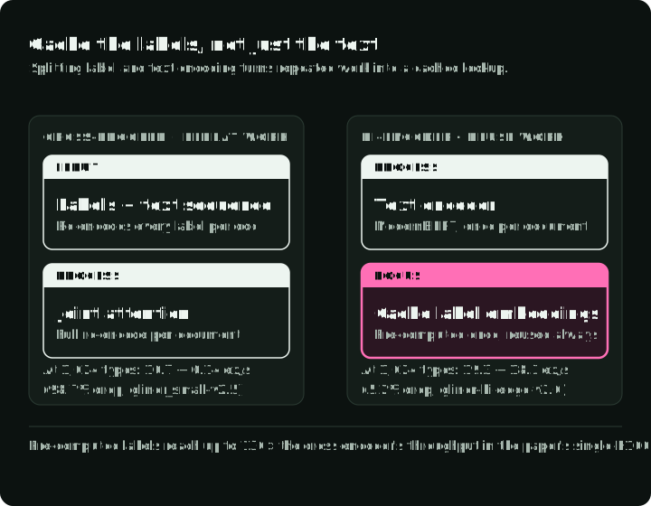
The text encoder uses ModernBERT (Ettin family), the label encoder uses sentence transformers (BGE or MiniLM). Spans and labels are scored via dot product. That split means entity type embeddings can be pre-computed once and cached. At inference, only the text needs encoding, and the label side becomes a cache read.
Four model sizes are available, all benchmarked on CrossNER (Stepanov et al., 2026, Table 1):
| Model | Parameters | CrossNER F1 | Throughput (H100) | With Pre-computed Labels |
|---|---|---|---|---|
| gliner-bi-edge-v2.0 | 60M | 54.0% | 13.64 ex/s | 24.62 ex/s |
| gliner-bi-small-v2.0 | 108M | 57.2% | 7.99 ex/s | 15.22 ex/s |
| gliner-bi-base-v2.0 | 194M | 60.3% | 5.91 ex/s | 9.51 ex/s |
| gliner-bi-large-v2.0 | 530M | 61.5% | 2.68 ex/s | 3.60 ex/s |
At 1,024 entity types, the pre-computed gliner-bi-edge-v2.0 bi-encoder loses only 5.2% throughput versus a single label (19.3 → 18.3 ex/s). The comparable gliner_small-v2.5 uni-encoder loses 98.7% (10.7 → 0.14 ex/s). In the paper’s single-H100, batch-size-1 tests across 64-, 256-, and 512-token inputs, the pre-computed bi-encoder reaches an up to 130× throughput advantage over gliner_small-v2.5. With 100 entity types on a single H100, the bi-encoder processes 1.96 million predictions per day versus 368K for the cross-encoder (Stepanov et al., 2026).
Accuracy holds up too. Bi-encoder-large hits 61.5% CrossNER F1, slightly ahead of the cross-encoder’s 60.9%. The authors recommend bi-base-v2.0 (194M) as the sweet spot, hitting 98% of the large model’s accuracy at 2.6x the speed (Stepanov et al., 2026).
from gliner import GLiNER

model = GLiNER.from_pretrained("knowledgator/gliner-bi-base-v2.0")

# Pre-compute embeddings for massive label sets — encode once, use forever
entity_types = ["person", "organization", "date"]  # Can be thousands or millions
entity_embeddings = model.encode_labels(entity_types, batch_size=8)

# Inference only encodes text — labels are a cached lookup
outputs = model.batch_predict_with_embeds(texts, entity_embeddings, entity_types)
Applications include biomedical NER against the UMLS ontology (4M+ concepts), enterprise taxonomies that evolve without model retraining, and entity linking via the companion GLiNKER framework.
LLMs as teachers: a $70 case study and a deployable pipeline
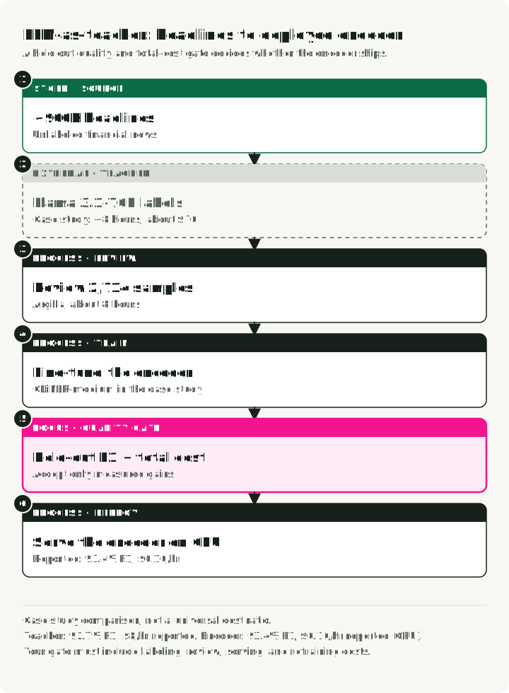
The LLM-as-teacher pattern separates expensive annotation from cheaper inference. Two published case studies show how teams have applied it under different conditions.
The CFM case study
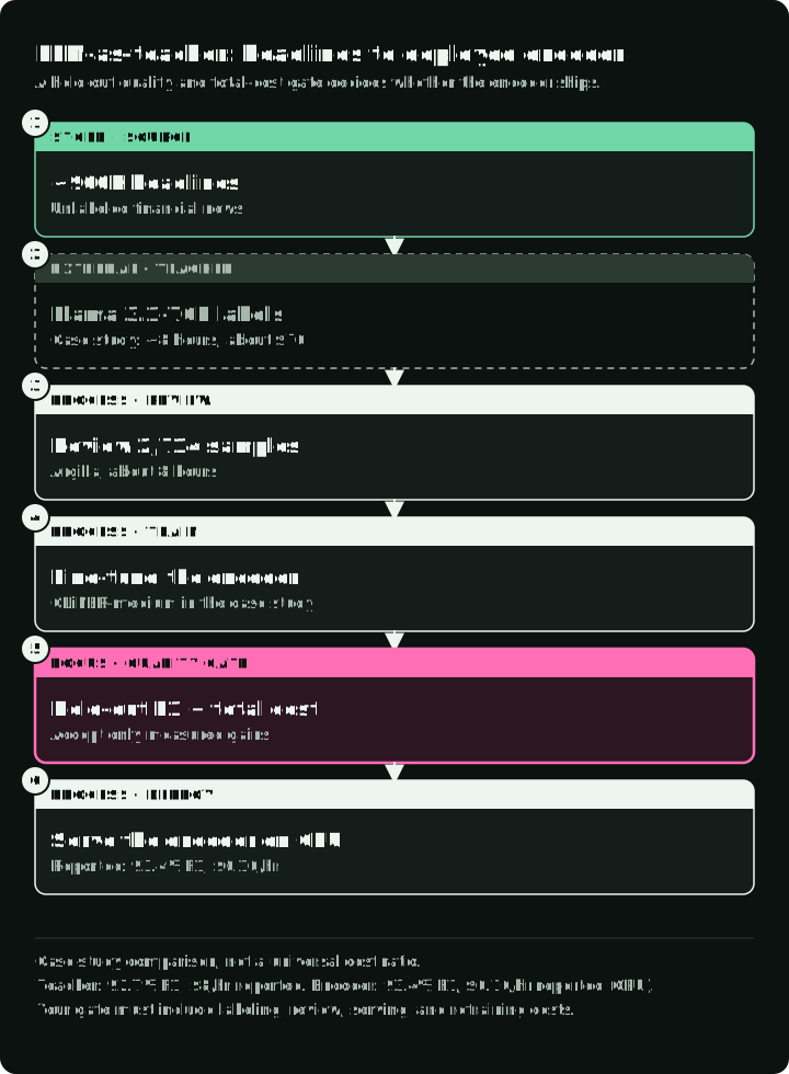
In a Hugging Face case study, Capital Fund Management extracted company names from roughly 900,000 financial news headlines. Zero-shot GLiNER scored 87.0% F1. The team used Llama 3.1-70B to annotate the dataset in roughly 8 hours for about $70, then reviewed 2,714 samples through Argilla in another 8 hours.
Fine-tuning GLiNER on this data reached 93.4% F1 in the case study, compared with the Llama-70B teacher’s 92.7%. The authors report $0.10 per hour on CPU for the fine-tuned model and $8 per hour for the teacher (CFM case study). Those figures describe one financial-news task and one infrastructure setup.
The Refuel AI study
Refuel AI’s technical report benchmarks LLM labeling across 8 NLP datasets, including CoNLL-2003. It reports 88.4% agreement with ground truth for GPT-4 (March 2023) and 86.2% for the human annotators in its setup, along with 20 times faster and 7 times cheaper labeling. Its ensemble routes easy examples to cheaper models and hard examples to GPT-4, reaching more than 95% agreement in the reported experiments (Refuel AI technical report). Treat these as vendor-reported results under that study’s annotation protocol.
A production pipeline
A practical production flow has six steps:
- Write annotation guidelines in natural language
- Create human-labeled validation and held-out test sets sized from entity prevalence, per-label slice requirements, and the desired confidence-interval width. A 50-200-document pilot can calibrate guidelines, but it is not a default production evaluation size.
- Use an LLM with a versioned prompt and explicit output schema to label bulk training data; retain the model version, prompt, and source text with each label
- Review a subset via Argilla or Label Studio
- Fine-tune a compact encoder (GLiNER, SpanMarker, RoBERTa)
- Deploy only if the encoder meets the quality gate and lowers measured total cost. CFM reported 16-80x lower hourly infrastructure cost in its setup; include annotation, review, serving, and retraining costs in your comparison.
The LLM can reduce the volume of manual annotation, but the team still owns the validation set, annotation guidelines, targeted review, and error analysis.
Where GLiNER fails and LLMs remain useful
The Sease benchmark (October 2025) tested GLiNER against GPT-4.1-mini on 30 query-parsing tasks. GPT-4.1-mini got 100% fully correct. GLiNER got 53% (16 of 30). But GLiNER responded in 0.08 seconds versus the LLM’s 1.21 seconds — 15x faster.
In this 30-task benchmark, GLiNER failed in three recurring patterns:
- Implicit entities: extracting “event” from “Elton John performed at Madison Square Garden” — no text literally says “event,” but the LLM infers “concert”
- Label phrasing sensitivity: “2022” scores 0.388 against “date” but 0.958 against “year” — small label changes cause large score swings
- Value mapping: GLiNER returns the exact surface text (“family houses”) instead of the canonical value (“Single family house”). An LLM can perform that normalization when its prompt and schema define the target values.
Nested and overlapping entities
GLiNER defaults to flat decoding, which suppresses overlapping spans. Its API also supports flat_ner=False, so nested predictions are possible, although quality depends on the checkpoint, labels, and domain data. Benchmark both decoding modes on a nested, span-level test set before choosing a specialized model.
Use GLiNER for explicit entity extraction and route cases requiring inference, reasoning, or mapping to predefined ontologies to an LLM. The routing threshold should come from a labeled domain set.
Evaluating NER: metrics, pitfalls, and test sets
A model can score 95% F1 on a curated test set and still fail on the document mix it sees after deployment. Build the evaluation set from the production distribution and keep slices for the rare formats and entity types that aggregate F1 can hide.
The core metrics
- Entity-level F1: The standard metric. A prediction is correct only if both the span boundaries and the type match ground truth exactly. This is what most papers report.
- Token-level F1: Scores each token independently. Inflates results because getting most of a long entity right earns partial credit. Prefer entity-level F1.
- Precision vs Recall: These often have asymmetric costs. For de-identification, recall matters more — missing a name is worse than over-redacting. For database extraction, precision matters more — false entries corrupt downstream analysis.
Common evaluation pitfalls
- Partial match inflation: “Bill” extracted when the gold label is “Bill Gates” — some scripts count this as a partial match. Use exact span matching unless you have a reason not to.
- Type confusion: “Microsoft” correctly identified as a span but labeled PERSON instead of ORG should score zero. Check your evaluation code handles this.
- Test set leakage: If test entities overlap with training entities, scores are inflated. Zero-shot benchmarks (CrossNER, Few-NERD) exist to test generalization.
- Uncontrolled label prompts: A short type name and a tested type description are different inputs. Version label descriptions, thresholds, checkpoint revisions, and decoding mode with the score.
- One-language zero-shot claims: Do not infer multilingual quality from English. OpenNER spans 36 corpora and 52 languages, and its baselines found no single model best in every language (Palen-Michel et al., 2025). In FiNERweb experiments, switching from English to target-language labels changed F1 by 0.02–0.09 depending on the setting (Golde et al., 2026). Test both label languages when the product uses local terminology.
- One run is a verdict: Report variation across random seeds where applicable, threshold sweeps, and repeated production samples. Small slice counts make a model ranking unstable.
Building a domain test set
For production evaluation, I recommend:
- Sample from production data, not curated examples. Include the messy documents your model will actually see.
- Size the test set for the estimate you need. Choose the count from entity prevalence, per-label slice sizes, and the desired confidence-interval width. Report bootstrap or analytic confidence intervals.
- Use at least two annotators on a calibration subset. Adjudicate disagreements and report a span-aware agreement measure. Agreement diagnoses ambiguity and guideline quality; it is not a model-performance ceiling.
- Stratify by difficulty — easy cases (clean text, standard types) and hard cases (ambiguous entities, jargon, noisy text).
- Keep privacy and fairness slices. For PII, report recall by PII type, language, locale, document format, and relevant demographic or name-origin slices. Minimize evaluator access to raw sensitive text, set retention limits, and review false negatives.
Continual NER needs an immutable regression set
Production taxonomies change. Add new types without silently changing what an old type means. Keep a versioned, immutable regression set for existing types, a separate test set for the new type, and a changelog for annotation-guideline changes. Report old-type and new-type scores separately before replacing a checkpoint. This is the simplest way to detect forgetting and taxonomy drift.
Production NER across four industries
These are selected industry examples with specific numbers under their reported conditions. The sources mix vendor-reported comparisons, company- or project-reported case studies, and peer-reviewed papers or preprints. Treat them as practical examples, not a maturity ranking.
Healthcare
John Snow Labs offers clinical entity models mapped to ICD-10, SNOMED CT, LOINC, and RxNorm. In its vendor-reported 48-document, six-class comparison, its token-level evaluation reported 96% F1, compared with Azure at 91%, AWS at 83%, and GPT-4o at 79%. The comparison remapped labels and excluded unmappable predictions. A separate provider-reported case study describes Providence St. Joseph Health processing 100,000-500,000 clinical notes daily.
In its 2025 project-reported review, the open-source OpenMed project reports 380+ biomedical NER models, 29.7 million Hugging Face downloads, and leading results on 10 of 12 public biomedical benchmarks.
Financial NER
The main use case: SEC filing extraction. John Snow Labs’ Finance NLP extracts 11+ entity types from 10-K/10-Q filings (addresses, tickers, fiscal years, stock exchanges). Peer-reviewed FinBERT-MRC variants hit 0.87-0.93 F1 on financial entity tasks. The hard parts are long documents and nested entities in complex financial instruments.
E-commerce
Peer-reviewed papers report that Walmart’s EAMT system (KDD 2023) trains on 965 million queries with about 60 entity labels and produced a 0.51% GMV lift in A/B tests. Home Depot’s TripleLearn framework (AAAI 2021) raised NER F1 from 69.5 to 93.3 through iterative training.
Cybersecurity
The peer-reviewed iACE system (CCS 2016) processed 71,000 articles from 45 security blogs, extracting 900K OpenIOC items at 95% precision and over 90% coverage. A project report for modern systems like CyNER describes combining DeBERTa (F1 >91%) with regex-based IOC heuristics. The CyberNER preprint’s 2025 unified dataset harmonizes four datasets into 21 STIX 2.1-aligned entity types, with RoBERTa hitting 0.736 F1.
Deployment optimization: from Python to lower-latency inference
The companion repo demonstrates GLiNER ONNX export and INT8 packaging. It records artifact sizes, but it does not reproduce the latency or F1 figures reported by external projects.
Native GLiNER serving
Before moving to a new runtime, test the project’s Ray Serve path. gliner[serve] provides dynamic batching, memory-aware batch sizing, multi-replica scaling, and an HTTP client. It can remove queueing overhead for a multi-user service while keeping the same model code. Benchmark queue latency, warm latency, throughput, and exact-span F1 under your request mix before comparing it with ONNX or Rust.
ONNX export
GLiNER has native ONNX conversion, and pre-converted models exist on Hugging Face (onnx-community/gliner_small-v2.1). Measure latency against the same PyTorch checkpoint, batch size, hardware, and warm-up protocol.
From scripts/02_onnx_export.py:
# Export with quantization
# python convert_to_onnx.py --model_path model/ --save_path onnx/ --quantize True

# Load the exported ONNX model
from gliner import GLiNER
model = GLiNER.from_pretrained("path/to/model", load_onnx_model=True)

entities = model.predict_entities(text, labels, threshold=0.5)
INT8 quantization
Dynamic quantization can reduce an ONNX model’s storage and memory requirements. The effect on latency and per-label F1 depends on the checkpoint and CPU, so the export script is packaging evidence rather than a deployment benchmark.
from onnxruntime.quantization import quantize_dynamic, QuantType

# Quantize weights dynamically, then evaluate the result
quantize_dynamic("gliner.onnx", "gliner_int8.onnx", weight_type=QuantType.QInt8)
gline-rs: Rust reimplementation
gline-rs (Apache 2.0) removes the Python runtime from the inference path. Its v0.9.0 token-mode benchmark on an Intel i9 with three labels reports 6.67 seq/s versus Python’s 1.61, and its RTX 4080 result reports 248.75 seq/s. Those are the project’s own conditions, not results reproduced by the companion repo. It supports span and token models, GPU/NPU via ONNX Runtime, and ships as a crate on crates.io.
use gliner::{GLiNER, TokenMode, Parameters, RuntimeParameters, TextInput};

let model = GLiNER::<TokenMode>::new(
    Parameters::default(), RuntimeParameters::default(),
    "tokenizer.json", "model.onnx")?;

let input = TextInput::from_str(
    &["My name is James Bond."], &["person", "vehicle"])?;
let output = model.inference(input)?;
// => "James Bond" : "person" (99.7%)
The fast-gliner package provides Python bindings via PyO3.
What the optimization evidence covers
| Path | Evidence available | Measure before deployment |
|---|---|---|
| ONNX export | Companion script exports a GLiNER checkpoint | Warm latency, throughput, and exact-span F1 |
| INT8 package | Companion script creates a dynamically quantized model | Artifact size, latency, and per-label recall |
| gline-rs | Project benchmark under its documented hardware/setup | Your model mode, labels, hardware, and batch |
Structured extraction: native schemas, Instructor, and local decoders
When you need more flexibility than encoder models offer — implicit entities, reasoning, ontology mapping — begin with the provider’s native schema mechanism. OpenAI supports strict json_schema response formats, Anthropic structured outputs supports JSON outputs and strict tool inputs, and the Gemini API supports a JSON Schema subset. A shared Pydantic or Zod model can describe the contract, but each provider accepts a different schema subset and has different refusal and complexity behavior.
Schema conformance makes parsing reliable. It does not prove that an extracted span exists in the source text or that a normalized value is correct. Validate field values, preserve offsets or quotations when possible, and score semantic accuracy on a labeled set.
Instructor wraps provider clients with Pydantic validation and optional retries after validation failures.
Adapted from the Instructor pattern in scripts/05_structured_extraction.py:
import instructor
from pydantic import BaseModel
from typing import List, Literal
from openai import OpenAI

class Entity(BaseModel):
    name: str
    label: Literal["PERSON", "ORGANIZATION", "LOCATION"]

class ExtractEntities(BaseModel):
    entities: List[Entity]

client = instructor.from_openai(OpenAI())
result = client.chat.completions.create(
    model="gpt-5.4-mini", temperature=0.0,
    response_model=ExtractEntities,
    messages=[{"role": "user", "content": "BioNTech SE acquired InstaDeep in the U.K."}])
# entities=[Entity(name='BioNTech SE', label='ORGANIZATION'), ...]
Outlines by dottxt takes a different approach: constrained token generation through finite-state machines. The decoder masks tokens that would violate the target grammar instead of waiting for a validation failure and retrying. An AWS overview cites 98% schema adherence versus 76% for post-generation validation. It separately repeats .txt Engineering’s claim of up to 5 times faster generation from its coalescence approach; the page does not publish enough methodology to treat both figures as one controlled benchmark.
import outlines
from transformers import AutoModelForCausalLM, AutoTokenizer

model_id = "microsoft/Phi-3-mini-4k-instruct"
model = outlines.from_transformers(
    AutoModelForCausalLM.from_pretrained(model_id),
    AutoTokenizer.from_pretrained(model_id),
)
result = model(
    "Extract entities from: BioNTech SE acquired InstaDeep in the U.K.",
    ExtractEntities,
)
LangExtract is useful when a generated field must be grounded in the source: it returns character intervals and supports hosted or local LLM backends. For self-hosted document extraction, NuExtract converts JSON schemas to templates and includes multimodal document models. Treat both as structured-extraction systems, not automatic replacements for span NER. Their field, offset, document-layout, and latency targets need their own tests.
The choice depends on where you run your models. Native schemas are the lowest-friction path for a supported provider. Instructor adds a provider-agnostic Pydantic validation and retry layer. Outlines constrains local generation against a schema. LangExtract prioritizes source grounding, while NuExtract targets self-hosted document extraction. All LLM paths still include autoregressive generation. Benchmark each path against an encoder on the same batch size, hardware, entity schema, and semantic-accuracy rubric.
The three-tier production architecture
I would route production NER by task shape rather than by one model ranking.
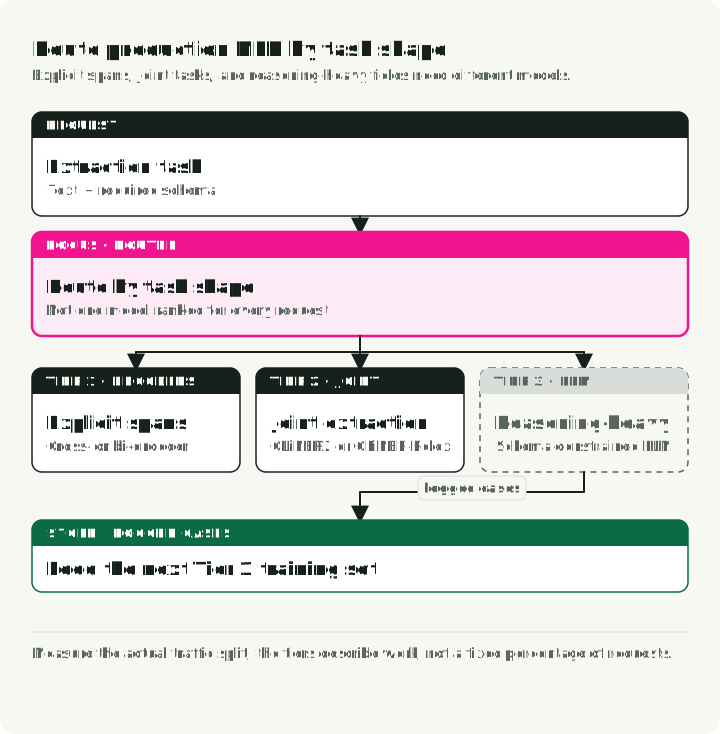
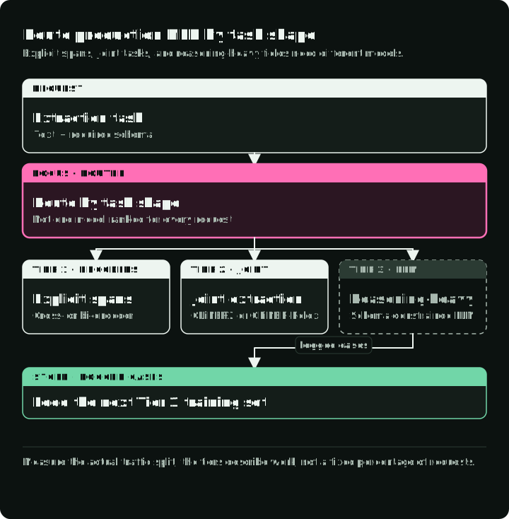
Tier 1: encoder models for explicit spans. Use a GLiNER cross-encoder for a small type inventory. When a large inventory is reused, compare the bi-encoder with cached type embeddings. Fine-tune through the LLM-as-teacher pipeline, then deploy with native serving, ONNX, INT8, or gline-rs only when that path passes the domain benchmark.
Tier 2: multi-task or relation extraction. When one request needs NER, classification, and hierarchical fields, test GLiNER2’s 205M-parameter shared model. When the central requirement is joint spans plus relations, test GLiNER-Relex. The GLiNER2 paper reports 130-208 ms CPU classification latency across its tested label counts; it is not evidence for the later relation API or for a different deployment.
Tier 3: LLMs for reasoning-heavy extraction. Route implicit entities, contextual inference, and ontology mapping to a native schema API or Instructor for cloud APIs, and to Outlines for local constrained output. Use LangExtract when source intervals are essential and NuExtract when the document itself is the input. Log these cases because they are candidates for the next Tier 1 training set.
The CFM case study gives one cost reference for Tier 1: 93.4% F1 at a reported $0.10 per hour on CPU, compared with 92.7% F1 and $8 per hour for its Llama-70B teacher. Recalculate that comparison with your hardware, teacher model, label set, and review cost.
Trade-offs and limitations
For each trade-off below, the useful questions are where it shows up and whether you can measure it before deployment.
LLM-as-teacher errors propagate. If the LLM consistently gets a specific entity type wrong (e.g., confusing subsidiary names with parent companies), the fine-tuned encoder inherits that bias. The fix is targeted human review — focus effort on entity types where the LLM’s confidence is low or inconsistent, not random sampling.
A valid schema can contain false facts. Native structured output, Instructor, and constrained decoders can make a response parseable. They cannot ensure that every field is grounded, that a span boundary is correct, or that a normalized value maps to the right record. Retain source evidence and validate semantics separately.
Quantization losses are checkpoint- and data-dependent. The companion creates a dynamically quantized INT8 artifact but does not measure its F1. Current GLiNER guidance recommends quantization-aware training when INT8 accuracy must be preserved. Compare the quantized and original checkpoints on exact-span F1 and per-label recall before deployment.
When the three-tier architecture is overkill. A single domain with stable entity types and enough labeled examples may need only a fine-tuned RoBERTa or spaCy pipeline. The three-tier pattern fits multiple domains, evolving entity types, or a measured mix of explicit and reasoning-heavy extraction. A narrow invoice pipeline that extracts names and dates may stop at Tier 1.
Bi-encoder quality varies by dataset. Joint encoding can help on some datasets, while the bi-encoder wins the paper’s CrossNER comparison and the uni-encoder edges it on CoNLL-2003. Benchmark both on the domain set; choose from measured exact-span quality, calibration, label count, and throughput rather than using “high stakes” as a model-family rule.
PII and multilingual claims require slices. A high aggregate score can hide a dangerous recall loss for a locale, name form, document layout, or rare PII class. Treat a privacy model as one defense in depth, set a false-negative response process, and re-evaluate when the taxonomy, language mix, or data source changes.
Key takeaways
- Use a compact encoder for explicit spans only after it passes a domain test set with per-type support and confidence intervals.
- Use GLiNER for changing label vocabularies. Compare its bi-encoder first when a large type inventory is reused; enable
flat_ner=Falseonly after measuring nested-span quality. - Use tested type descriptions for hard zero-shot claims, and test English and localized label wording separately for multilingual products.
- Keep OCR, NER, relation extraction, and entity linking as distinct evaluation stages even when one model exposes several tasks.
- Treat an LLM teacher as an annotation proposal system. Human guidelines, adjudication, immutable regression sets, and a held-out test set remain required.
- Use native schemas for supported LLM providers, but validate semantic correctness and source grounding separately from JSON validity.
- Benchmark native serving, ONNX, quantization, and Rust paths separately and together. Never multiply unmeasured speedups.
References
Papers
- GLiNER: Generalist Model for Named Entity Recognition using Bidirectional Transformer - Zaratiana et al., NAACL 2024. The foundational span-entity matching architecture.
- GLiNER2: An Efficient Multi-Task Information Extraction System with Schema-Driven Interface - Zaratiana et al., EMNLP 2025 System Demonstrations. Unifies NER, classification, and hierarchical extraction; current releases later added relation extraction.
- GLiNER Bi-Encoder: Scalable Named Entity Recognition with Bi-Encoder Architecture - Stepanov et al., February 2026. Decoupled encoding for million-label scale.
- GLiNER-Relex: A Unified Framework for Joint Named Entity Recognition and Relation Extraction - Stepanov et al., 2026. Joint, zero-shot entity and relation extraction.
- GLiNER2-PII: A Multilingual Model for Personally Identifiable Information Extraction - Zaratiana et al., 2026. 42 PII types at character-span resolution.
- ZeroNER: Fueling Zero-Shot Named Entity Recognition via Entity Type Descriptions - Cocchieri et al., ACL 2025. Hard zero-shot evaluation with type descriptions.
- OpenNER 1.0: Standardized Open-Access Named Entity Recognition Datasets in 50+ Languages - Palen-Michel et al., EMNLP 2025. 36 corpora, 52 languages, and multi-ontology baselines.
- FiNERweb: Datasets and Artifacts for Scalable Multilingual Named Entity Recognition - Golde et al., EACL 2026. Multilingual labels and transfer evaluation.
- UniNER: Universal NER using Large Language Models - Zhou et al., ICLR 2024. LLM-based universal NER via distillation from ChatGPT.
- NuNER: Entity Recognition Encoder Pre-training via LLM-Annotated Data - Bogdanov et al., EMNLP 2024. Shows 125M parameters suffice with LLM-generated training data.
Industry papers
- EAMT: Entity-Aware Multi-Task Learning for Query Understanding - Walmart, KDD 2023. 965M queries, 0.51% GMV lift.
- TripleLearn: End-to-End NER for E-Commerce Search - Home Depot, AAAI 2021. F1 from 69.5 to 93.3.
- iACE: Automatic Collection of Cyber Threat Intelligence - CCS 2016. 71K articles, 900K IOCs.
- CyberNER: A Harmonized STIX Corpus for Cybersecurity NER - 21 STIX 2.1-aligned entity types.
- FinBERT-MRC: Financial NER via Machine Reading Comprehension - 0.87-0.93 F1 on financial entity tasks.
Case studies
- CFM Case Study: Fine-tuning GLiNER for Financial NER - Capital Fund Management’s $70 LLM labeling pipeline achieving 93.4% F1.
- Refuel AI: LLM Labeling Technical Report - GPT-4 achieving 88.4% annotation agreement, exceeding human annotators.
- Sease: GLiNER as an Alternative to LLMs for Query Parsing - Where GLiNER fails and LLMs are still needed.
- John Snow Labs: Medical Text De-Identification Benchmark - 96% F1 PHI detection comparison across providers.
- OpenMed: Year in Review 2025 - 380+ biomedical NER models, 29.7M HuggingFace downloads.
Tools and frameworks
- ner-field-guide demo repo - Companion demos for this article: GLiNER quickstart, ONNX export, LLM-as-teacher, and structured extraction.
- gline-rs: Rust reimplementation of GLiNER - 4.1x CPU speedup over Python, Apache 2.0 licensed.
- GLiNER serving - Ray Serve path with dynamic batching and multi-replica deployment.
- spaCy English pipelines - Versioned closed-label pipeline metrics.
- Microsoft Presidio - PII analysis and anonymization with custom recognizers.
- Instructor - Structured LLM extraction via Pydantic models.
- Outlines - Constrained token generation via FSMs, with a reported schema-adherence benchmark.
- LangExtract - Source-grounded structured extraction with character intervals.
- NuExtract - Self-hosted, schema-to-template document extraction.
- OpenAI Structured Outputs - Strict JSON-schema response format reference.
- Anthropic Structured Outputs - JSON outputs and strict tool inputs.
- Gemini Structured Outputs - JSON Schema subset for structured responses.
- AWS: Structured Output with Outlines - 98% schema adherence benchmark.