LLM Engineering Guide: 45 Concepts for Production Systems

An LLM service can miss its latency SLO because decode is limited by memory bandwidth, because the KV cache has consumed the batch budget, or because the queue is masking both. A fine-tuning run can fail for a different version of the same reason: model state no longer fits the hardware. The right fix follows from the bottleneck, not from the longest list of techniques.
This is a reference for engineers who already know basic ML and systems concepts, and need to connect a production symptom to the relevant part of the stack. It covers 45 concepts across hardware, inference, training, deployment, applications, and operations. Use an entry to identify the mechanism, its practical consequence, and the condition that limits the cited result; then use the linked deep dive or your own benchmark to make the decision.
A note on scope
This is a reference, not a linear tutorial. Start with the part that matches the decision in front of you.
| Part | Topics | Sections |
|---|---|---|
| I — Hardware foundations | Roofline model, GPU memory, hardware glossary | 1–3 |
| II — Inference fundamentals | Latency, throughput, KV cache, attention, quantization | 4–9 |
| III — Inference optimizations | CUDA kernels, FlashAttention, batching, PagedAttention, speculative decoding | 10–17 |
| IV — Model architecture | Transformer internals, decoder-only, MoE, tokenization, context windows | 18–22 |
| V — Training and alignment | Pretraining, LoRA, mixed precision, ZeRO, scaling laws, RLHF/DPO/GRPO, distillation | 23–32 |
| VI — Scaling and deployment | Parallelism, serving frameworks, GPU selection, routing | 33–36 |
| VII — Applications | Embeddings, RAG, agents, prompt engineering | 37–40 |
| VIII — Production operations | Rate limiting, failure modes, monitoring, cost, capacity planning | 41–45 |
How to use this guide as a hub
This page is deliberately broad. Use it as the map, then jump to the deeper posts when the decision becomes concrete.
| If you are deciding… | Start with | Then read |
|---|---|---|
| How to serve a model | Inference fundamentals and deployment | LoRAX Serving Guide |
| Whether to fine-tune | Training and alignment | LLM Fine-Tuning Guide |
| How retrieval fits into an app | Embeddings and RAG | RAG Evaluation Metrics |
| How agent systems work | Agents and prompt engineering | AI Agent Reasoning Loops |
| How to rank search results | Embeddings and reranking | Search Ranking Stack |
Start with the bottleneck, use the smallest stack that exposes it, benchmark the real workload, and add complexity only where the numbers justify it.
Part I — Hardware foundations
Arithmetic intensity, the GPU memory hierarchy, and the hardware terms in this part explain many of the choices later in the guide.
1. Memory-bound vs compute-bound and the roofline model
The starting point for LLM performance is arithmetic intensity: for every byte of data the GPU loads from memory, how many useful calculations does it perform? That ratio decides whether an operation is compute-bound (waiting on the processor) or memory-bound (waiting on data to load).
Every GPU has a “critical intensity” threshold where its peak compute throughput equals its memory bandwidth. For an NVIDIA H100 SXM using dense BF16 or FP16 Tensor Cores (989 TFLOPS; the 1,979-TFLOPS specification assumes structured sparsity):

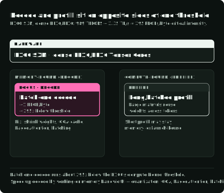
Batch-one decode and long or sufficiently batched prefill commonly sit on opposite sides of this threshold:
- Decode is memory-bound. Generating tokens one by one means loading the multi-gigabyte weight matrix from memory to multiply it against a single new token. In a simplified dense 16-bit, batch-one analysis, the operation has about 1 FLOP/byte, roughly 295x below the H100 roofline threshold. That gap explains why decode cannot approach peak compute throughput in this regime.
- Long or sufficiently batched prefill is often compute-bound. Processing many prompt tokens reuses weights across large matrix multiplications, which can push arithmetic intensity above the roofline threshold. Short prompts and small batches may instead be limited by memory traffic or kernel-launch overhead.
So to speed up decode, work on memory bandwidth: shrink the weights with quantization, reduce KV memory overhead with GQA and PagedAttention, and raise intensity with batching. For long or well-batched prefills, faster matrix computation and lower-precision compute may help; profile short-prefill workloads separately.
2. GPU memory hierarchy
A GPU has four memory layers, arranged like a pyramid: a large but slow main memory (HBM) at the bottom, tiny but very fast registers at the top. Moving data through this hierarchy is a major performance constraint.
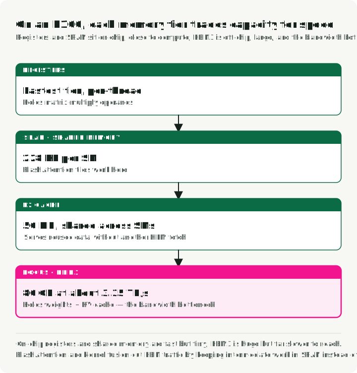
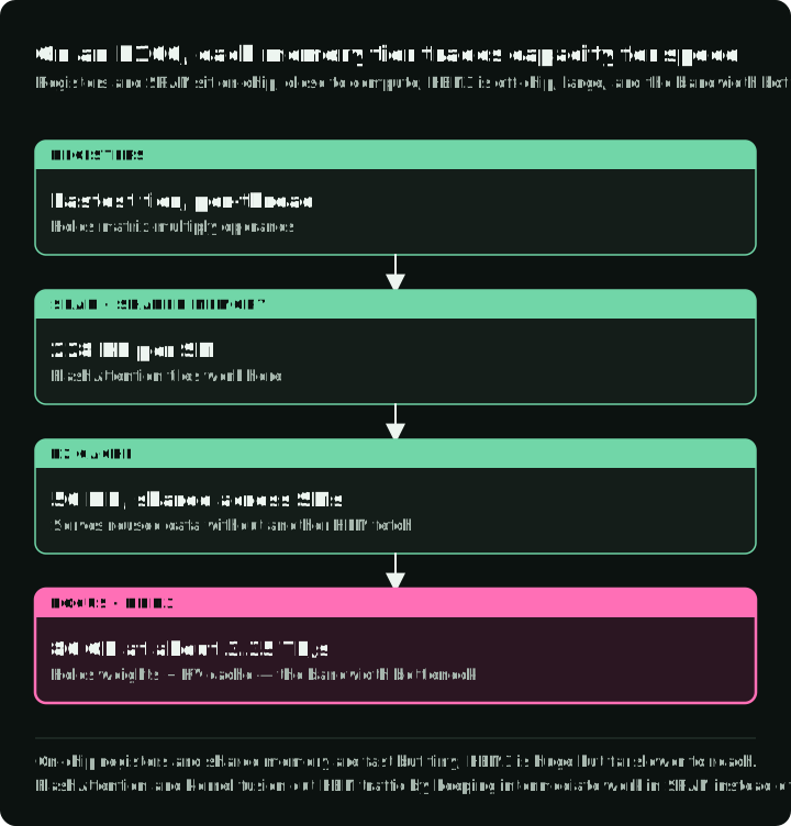
From fastest to slowest on an H100:
- Registers are the fastest memory and attach directly to processing threads. For Hopper’s WGMMA, matrix A can come from registers or shared memory, while matrix B comes from shared memory.
- SRAM (shared memory) is fast on-chip working memory local to each SM.
- L2 cache is a 50 MB shared layer. It can serve data reused across SMs without another HBM fetch.
- HBM3 is the 80 GB main memory that holds model weights and the KV cache, with ~3.35 TB/s of bandwidth.
FlashAttention and kernel fusion reduce HBM traffic by retaining or combining intermediate work on chip. PagedAttention targets a different problem: it maps logical KV blocks to noncontiguous physical GPU-memory blocks, reducing fragmentation and enabling block sharing.
3. GPU hardware glossary
The terms below show up throughout the rest of the guide.
HBM (High Bandwidth Memory) stacks DRAM dies connected by through-silicon vias (TSVs) next to the GPU die. Generations include HBM2e (A100, 2 TB/s), HBM3 (H100, 3.35 TB/s), and HBM3e (H200/B200, 4.8–8 TB/s). HBM bandwidth is a direct constraint on TPOT in memory-bound decode regimes.
GDDR (Graphics DDR) is traditional graphics memory used in consumer and workstation GPUs such as the RTX 4090 and L40S. It has lower bandwidth than HBM but costs less per GB. GDDR6X on the RTX 4090 delivers about 1 TB/s versus the H100’s 3.35 TB/s of HBM3 bandwidth.
An SM (Streaming Multiprocessor) is the basic compute block in an NVIDIA GPU. Each SM contains CUDA cores, Tensor Cores, shared memory, and a warp scheduler. The H100 has 132 SMs; the A100 has 108.
Tensor Cores are specialized matrix-multiply-accumulate units inside each SM. They accelerate the mixed-precision matmuls that dominate transformer computation. H100 SXM Tensor Cores deliver 494.5 dense or 989 sparse TF32 TFLOPS; always include the precision and sparsity mode when comparing this figure.
CUDA Cores are general-purpose floating-point and integer units. They handle element-wise operations, activation functions, and other non-matrix work while Tensor Cores run supported matrix operations.
A warp is a group of 32 threads that execute in lockstep on an SM, making it NVIDIA’s smallest scheduling unit. Warp specialization assigns different warps to data movement and computation so the tasks can overlap.
NVLink is NVIDIA’s high-speed GPU-to-GPU interconnect within a node. NVLink 4.0 on H100 delivers 900 GB/s bidirectional bandwidth; NVLink 5.0 on B200 reaches 1.8 TB/s. This bandwidth matters for tensor parallelism because GPUs exchange partial results at every transformer layer.
InfiniBand is a high-speed network fabric for inter-node communication. ConnectX-class InfiniBand adapters provide the inter-node fabric for pipeline-parallel or distributed-training traffic; bandwidth depends on the adapter and port configuration.
RDMA (Remote Direct Memory Access) lets a device access memory on another machine without routing the data path through either CPU. GPUDirect RDMA supports direct GPU-to-GPU transfers across nodes, including KV-cache transfers in disaggregated serving.
NVMe (Non-Volatile Memory Express) is the SSD interface used for KV-cache offloading and ZeRO-Infinity parameter offloading when GPU and CPU memory are insufficient. Sequential bandwidth depends on the drive and workload, and it remains far below HBM bandwidth.
TFLOPS and PFLOPS are trillions and quadrillions of floating-point operations per second. One TFLOPS equals FLOPS. H100 reaches 989 sparse TF32 tensor TFLOPS, while FlashAttention-3 reports about 1.2 PFLOPS in FP8; those values use different formats and should not be compared as if they were one metric.
Part II — Inference fundamentals
Inference turns a model into a user-visible service. The following concepts separate work that delays the first token from work that slows every later token, and expose the memory limits behind both.
4. Latency: TTFT, TPOT, and percentiles
Time to First Token (TTFT) is the end-to-end delay from request submission to the first output token. It includes queueing, tokenization, scheduling, prompt prefill, the first decode step, and network delivery. Longer prompts usually increase the prefill component, but any of these stages can dominate. Targets are product-specific; MLPerf Inference v5.0 uses a P99 TTFT limit of 450 ms for its Llama 2 70B interactive scenario.
Time Per Output Token (TPOT) is the average interval between consecutive tokens after the first. It maps to the decode phase. Batch-one or low-intensity decode is usually memory-bandwidth-bound, while sufficiently large batches can become compute-bound:
This definition requires at least two output tokens; TPOT is undefined for a one-token response.
Average adult English silent reading speed is about 238 words per minute for non-fiction (Brysbaert, 2019). Streaming targets should still come from product testing; MLPerf uses a P99 TPOT limit of 40 ms for its interactive scenario.
P50 vs P99 latency matters because the median hides the tail. A system with a good P50 and a bad P99 may have batching, preemption, queueing, or workload-skew problems; traces are needed to distinguish them.
5. Throughput: tokens per second and the latency tradeoff
Throughput is measured in output tokens per second across concurrent requests. Requests per second is weaker on its own because a 10-token response and a 1,000-token response have very different costs. Published benchmark numbers vary with model, precision, hardware, prompt and output lengths, concurrency, and SLO. Compare vLLM, SGLang, and TensorRT-LLM with one harness rather than combining their headline results.
The tradeoff: at low concurrency, each request gets great latency but the GPU is underutilized. Increasing batch size raises throughput almost linearly until compute saturates, after which latency climbs sharply. Goodput, the rate of requests per second that meet your SLO targets, connects raw throughput to what users actually experience.
6. KV cache: the bottleneck behind most other bottlenecks
During autoregressive generation, each new token attends to every previous token. The KV cache stores the Key and Value projections from every token at every layer to avoid recomputation. Without it, generating token would require re-running the model over all previous tokens.
The KV cache can become the dominant variable memory pressure at long sequence lengths or high concurrency because it grows linearly with sequence length, batch size, and layer count:
where:
- = number of layers
- = number of KV heads
- = head dimension
- = sequence length
- = batch size
- = bytes per cached element, set by the KV-cache precision
Concrete examples with FP16 and batch size 1: Llama 3.1 8B at 8,192 tokens uses ~1.0 GB of KV cache; at 128K tokens, 16 GB. Llama 3.1 70B at 128K tokens needs ~40 GB for a single sequence, half of an H100’s VRAM. At high concurrency or long context, KV cache can exceed model weight memory; the result depends on sequence length, active batch size, KV precision, and the number of KV heads. Naive implementations waste 60–80% of the allocated KV memory to fragmentation, which is the problem PagedAttention was built to solve.
The main optimizations are GQA (fewer KV heads), KV cache quantization (FP8/INT8), PagedAttention (block-based allocation with <4% waste), and offloading KV cache to CPU or NVMe.
7. Prefill vs decode: two phases, two bottlenecks
The prefill phase processes the input prompt in parallel and populates the KV cache. Long or sufficiently batched prefills often become compute-bound because they use large matrix multiplications; short prefills may remain limited by memory traffic or kernel-launch overhead. Prefill contributes to time to first token (TTFT), alongside queueing, tokenization, scheduling, the first decode step, and network delivery. The decode phase generates one token at a time. Each step reads model weights and the KV cache from HBM, making batch-one decode memory-bandwidth-bound and the main driver of time per output token (TPOT).


Chunked prefill splits the prompt into fixed-size chunks instead of processing it all at once. A scheduler can interleave those chunks with decode work so one long prompt does not monopolize an iteration. Sarathi-Serve reports better throughput-latency trade-offs in its tested workloads, but the gain depends on the model, hardware, request-length distribution, chunk size, and comparison baseline. Extra scheduling and smaller kernels can raise TTFT for the new request.
Disaggregated serving places prefill and decode on separate GPU pools, allowing each pool to target a different bottleneck. Splitwise and DistServe describe the pattern. The pools transfer KV-cache data over a fast interconnect such as RDMA, so communication cost becomes part of the design.
8. GQA and MQA: shrinking the KV cache
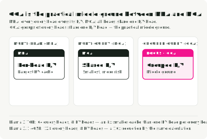
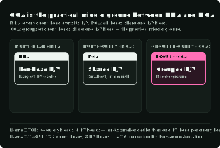
Standard Multi-Head Attention (MHA) gives every query head its own K and V head. Multi-Query Attention (MQA) shares a single KV head across all query heads, which is an extreme reduction. Grouped-Query Attention (GQA) is the practical middle ground: groups of query heads share one KV head.
Llama 3 70B uses 64 query heads but only 8 KV heads, an 8x KV cache reduction versus the same architecture with one KV head per query head. Llama 3.1 405B uses 128 query heads and 8 KV heads, a 16x reduction by the same calculation (Meta, 2024). Ainslie et al. report GQA quality close to MHA in their tested models while approaching MQA speed. A smaller KV cache can support larger batches, but the realized latency and throughput gain still depends on the kernel and workload.
9. Quantization: trading bits for speed and memory
Quantization reduces the precision of model weights and/or activations. The core tradeoffs:
| Format | Bits | Weight memory (7B model) | Quality note |
|---|---|---|---|
| FP16/BF16 | 16 | ~14 GB | Baseline for comparison |
| FP8 | 8 | ~7 GB | Hardware-native on Hopper; evaluate model |
| INT8 | 8 | ~7 GB | Calibration and kernel dependent |
| INT4 | 4 | ~3.5 GB | Largest compression; evaluate carefully |
AWQ (Activation-Aware Weight Quantization) identifies salient weight channels from activation magnitudes and applies per-channel scaling to protect them. Its calibration needs depend on the model and configuration; in one OPT-6.7B INT3-g128 comparison, AWQ used 16 calibration sequences while GPTQ used 192. Report both the sequence count and sequence length in a reproducible setup. GPTQ uses approximate second-order information for layer-wise quantization. bitsandbytes can quantize during model loading without a separate preprocessing pass; its NF4 format powers QLoRA fine-tuning. FP8 on Hopper-class hardware halves weight memory relative to FP16/BF16, but quality and speed still depend on the model, calibration, and kernel.
The serving kernel can matter as much as the quantization algorithm. Section 10 gives a bounded Marlin result and explains why the gain depends on the serving configuration.
Part III — Inference optimizations
The optimizations in this part solve different constraints. FlashAttention reduces attention’s HBM traffic; PagedAttention improves KV allocation; continuous batching prevents finished sequences from holding batch capacity.
10. CUDA kernels and kernel fusion
A CUDA kernel is a function written for the GPU that runs in parallel across thousands of threads. When the CPU calls a kernel, the GPU distributes the work across its SMs: each SM runs multiple warps of 32 threads, and each thread processes a slice of the data. Every operation in LLM inference, from matrix multiplication to token sampling, is ultimately a kernel launch. A single forward pass through a 70B model triggers hundreds to thousands of kernel launches, and the gap between a naive kernel and an optimized one can decide whether your system meets its latency SLO.
The main kernel categories in LLM serving:
- GEMM kernels for matrix multiplication, which dominate both prefill and decode compute.
- Attention kernels like FlashAttention that tile computations to stay in SRAM instead of spilling to HBM.
- Fused kernels that combine multiple operations (such as add + layer norm or QKV projection) into a single launch to skip the intermediate HBM round-trips.
- Sampling kernels that convert logits to token IDs via top-k, top-p, or temperature sampling.
Kernel quality can determine whether compressed weights deliver a speedup. The Marlin paper reports up to 2.8x end-to-end speedup over its FP16 baseline for tested weight-only INT4 vLLM configurations. That result is specific to the paper’s models, GPUs, batch sizes, and serving setup, so it is not a universal INT4 gain.
Triton lowers the barrier to writing custom kernels by exposing GPU programming through Python instead of raw CUDA C++, which puts kernel-level optimization within reach of ML engineers and not only GPU specialists. Most of the optimizations later in this part (FlashAttention, fused kernels, PagedAttention) are either better kernels or smarter ways to orchestrate kernel launches.
Kernel fusion combines sequential operations into one GPU kernel and skips intermediate HBM writes. Common fusions include QKV projection, attention plus softmax, add plus RMSNorm (FlashNorm), and SwiGLU activation (DeepFusionKernel). Triton makes these kernels accessible through Python. The exact launch-count and utilization gains depend on the model graph, compiler, GPU, and serving framework, so profile the deployed stack rather than relying on a universal percentage.
11. FlashAttention: tiling attention to live in SRAM
Standard attention materializes the full attention matrix in HBM, which costs memory and produces a lot of memory traffic. The idea behind FlashAttention is to never materialize this matrix at all. It tiles the Q, K, V matrices into blocks that fit in SRAM, computes partial attention within each tile, and merges results using an online softmax (incrementally tracking the running max and sum across blocks). Memory drops from to , and HBM reads drop by an order of magnitude.
Each version targets the bottleneck of its GPU generation:
- FlashAttention v1 (A100, 2022) proved the tiling plus online-softmax idea works. The paper reported a 2–4x speedup over standard attention, but only 25–40% GPU utilization because kernel scheduling left many SMs idle.
- FlashAttention v2 (A100, 2023) reworked the parallelism to split across the sequence dimension rather than batch and heads. It reached 50–73% utilization on A100, roughly 2x faster than v1.
- FlashAttention v3 (H100 Hopper, 2024) added warp specialization (separate warps for data movement vs. math) and GEMM-softmax pipelining to overlap memory loads with computation. The paper reports up to 740 TFLOPS/s in FP16 (75% utilization) and close to 1.2 PFLOPS/s in FP8 on H100. NeurIPS 2024 spotlight.
- FlashAttention v4 (B200 Blackwell, 2026) addresses a new bottleneck: on Blackwell, tensor core throughput scales so fast that non-matmul operations (softmax exponentials, rescaling) become the limiter. FA4 software-emulates the exponential with polynomial approximations on FMA units, uses conditional rescaling to reduce overhead, and stores intermediates in Blackwell’s dedicated tensor memory (TMEM) instead of registers. The paper reports about 1.6 PFLOPS on B200 in BF16, 1.3x faster than cuDNN 9.13 and 2.7x faster than Triton in its tests.
12. FlashDecoding: parallelizing the decode bottleneck
Standard FlashAttention keeps the GPU busy by splitting work across batch size and query length. During decode the model generates exactly 1 token at a time (query length = 1). If the batch size times the number of attention heads is less than the GPU’s total SM count (108 on an A100), most of the GPU sits idle while a few units grind sequentially through the token history.
FlashDecoding solves this by adding a new parallelization dimension: the KV sequence length itself. It chops the KV cache into smaller chunks and distributes them across all the otherwise-idle GPU processors to evaluate in parallel, then merges their partial computations with a log-sum-exp reduction.
In Stanford’s batch-one CodeLlama-34B benchmark, with sequence lengths from 512 to 64K tokens, FlashDecoding reached up to an 8x end-to-end speedup over the tested baselines and kept attention latency nearly constant through 64K. The result is bounded to that hardware and benchmark rather than a general decode guarantee.
13. Continuous batching vs static batching
Static batching waits for every sequence in a batch to finish before starting the next, so short sequences waste GPU cycles idling after they hit end-of-sequence. Continuous batching (introduced by the Orca paper, OSDI 2022) operates at iteration-level granularity: at each decode step, completed sequences are removed and new ones inserted.
In Anyscale’s OPT-13B benchmark, optimized static batching reached 4x its naive baseline, continuous batching reached 8x, and vLLM with continuous batching plus PagedAttention reached 23x (Anyscale, 2023). Continuous batching also increases pressure on KV allocation, which is why it is commonly paired with paged memory management.
14. PagedAttention: virtual memory for KV cache
vLLM’s PagedAttention applies the OS virtual-memory idea to KV cache management. The KV cache is split into fixed-size blocks (typically 16 tokens), blocks are allocated on demand as tokens are generated, and logical (sequential) positions map to physical (scattered) memory locations through block tables. Multiple requests that share a prefix (system prompts, beam search) can point to the same physical blocks.
Earlier systems wasted 60–80% of KV cache memory to fragmentation and pre-allocation. PagedAttention drops that to <4%, which lets throughput rise 2–4x at the same latency and up to 24x over HuggingFace Transformers (vLLM Blog, 2023).
15. Speculative decoding: multiple tokens per forward pass
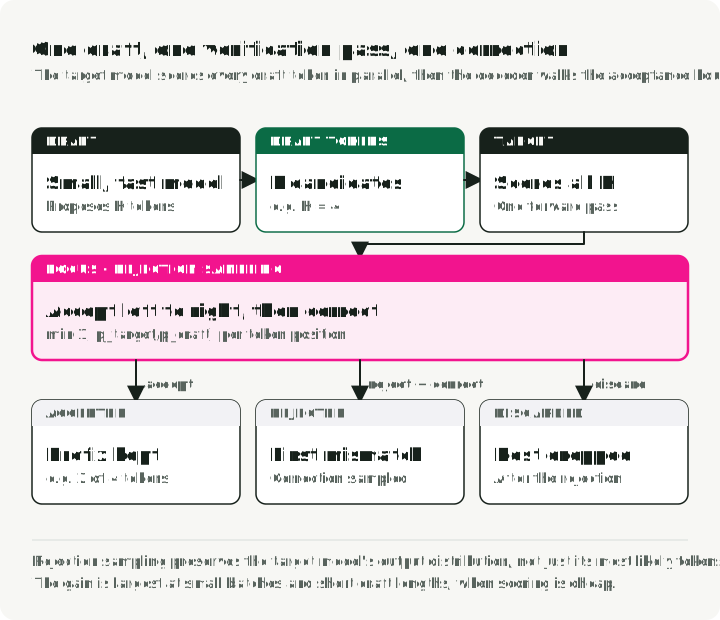
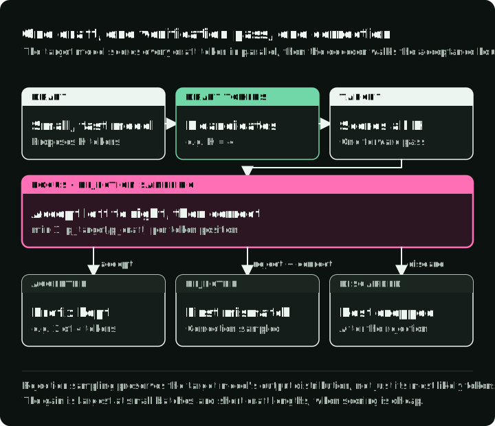
In speculative decoding, a small draft model generates candidate tokens, then the large target model scores all positions in one forward pass. The decoder accepts draft tokens from left to right with probabilities derived from the target and draft distributions. After the first rejection, it samples a correction from the residual target distribution and discards the remaining draft tokens. This modified rejection-sampling step preserves the target model’s output distribution within hardware numerics; exact token matching alone does not.
The gain is most plausible at small serving batches and short draft lengths, when scoring the draft is dominated by weight, KV-cache, or communication traffic rather than the extra token compute. The original speculative-sampling paper reported a 2–2.5x decoding speedup for its tested 70B Chinchilla setup; EAGLE-3 reported up to 6.5x in its tests. Variants include Medusa (extra prediction heads, no separate model), prompt lookup decoding (n-gram matching against the input without a separate draft-model forward pass), and EAGLE (feature-level extrapolation).
At high batch sizes, extra draft and verification work can erase the gain. Speculative decoding is most promising when the serving batch is small enough and draft acceptance is high; benchmark the full serving loop rather than the verification kernel alone.
16. Prefix caching and KV cache reuse
Instead of throwing away the KV cache when a request finishes, prefix caching keeps it around for reuse on new requests that share the same prefix tokens. That cuts redundant prefill for system prompts, few-shot examples, RAG context, and multi-turn conversation history.
vLLM’s Automatic Prefix Caching hashes KV blocks and uses a global hash table for lookup. SGLang’s RadixAttention maintains a radix tree of cached KV tensors with token-level granularity. Both depend on repeated token-identical prefixes, so report hit rate alongside latency or throughput.
17. Streaming in practice
Streaming sends tokens to the client as they are generated instead of waiting for the full response. Many serving frameworks expose it via Server-Sent Events: the client opens a long-lived HTTP connection, and the server pushes each token or token batch as a data: event. TTFT determines when the user first sees output; TPOT helps determine how smooth it feels. Set the target through product testing and the chosen interaction model.
On the client side, streaming forces buffering decisions. Rendering token by token can cause visual jitter, especially with markdown or code blocks that need multi-token context to format correctly. Common patterns are word-level buffering (accumulate tokens until a whitespace boundary), line-level buffering (wait for a newline before rendering), and adaptive buffering (render immediately for prose, buffer for code blocks). In the OpenAI Chat Completions API, stream_options: {"include_usage": true} adds a final usage chunk before the data: [DONE] message. OpenAI-compatible servers may differ, so verify the selected implementation.
Chunked prefill is one way to keep long prefills from stalling token delivery for concurrent users. Decode-priority scheduling can protect in-flight requests, while disaggregated serving isolates prefill and decode on separate GPU pools.
Part IV — Model architecture
Architecture sets the memory footprint, attention behavior, and training dynamics that the serving and training sections work around.
18. Transformer architecture essentials
A modern decoder-only transformer (GPT, Llama) is a stack of identical layers, each with two sub-blocks: attention and feed-forward. Every sub-block is wrapped with a residual connection and normalization. The key components:
Multi-Head Attention lets each token weight information from the tokens visible under the attention mask. The input is projected into three matrices: Queries (what am I looking for?), Keys (what do I contain?), and Values (what information do I carry?). Attention scores are then computed as:
The dot product measures similarity between every pair of tokens. Dividing by keeps the dot products from growing too large (which would push softmax into regions with vanishing gradients). The softmax converts scores to probabilities, and multiplication by produces a weighted combination of value vectors. Running this across multiple heads in parallel lets the model attend to different relationships at the same time (one head for syntax, another for coreference, and so on).
The Feed-Forward Network (FFN) transforms each token representation independently after attention mixes information across tokens. Modern LLMs often use SwiGLU instead of the original two-matrix ReLU FFN:
SwiGLU has three weight matrices, versus two for a ReLU FFN, and uses smooth Swish. Llama, Mistral, and Qwen use it; Gemma uses an approximate GeGLU. The familiar two-thirds rule applies to a conventional full-MHA block with : its two FFN matrices contribute about parameters, versus about for attention. It is not a general estimate for SwiGLU/GQA architectures. In Llama 3 8B, , , and eight key/value heads make the FFN M parameters per layer, versus about 42M attention-projection parameters: about 81% of those projection weights, before embeddings and normalization.
Residual connections add each sub-block’s output back to its input: . The skip path improves signal and gradient propagation through deep stacks.
RMSNorm is common in modern LLM families. LayerNorm re-centers by subtracting the mean and re-scales by the standard deviation. RMSNorm skips mean subtraction and only re-scales; its paper reports 7–64% speedups across the tested models without a performance penalty in those experiments. Pre-norm placement, which normalizes before attention or the FFN, is also common because it improves gradient stability.
Parameter count estimation for a decoder-only model:
where is vocabulary size, is hidden dimension, and is layer count. The term is the input embedding matrix; the term approximates the attention and FFN weights in each layer. For Llama 3 8B (, , ), the estimate is about parameters. The published 8.03B total is higher because the approximation omits architectural details such as the exact FFN width and the separate output projection.
19. Decoder-only models for general-purpose generation
The original Transformer (2017) had both an encoder and a decoder. Since then, the field split into three architectural families, and one became the default for generative AI.
Encoder-only models (BERT, RoBERTa) use bidirectional attention: every token attends to every other token in both directions. That produces rich representations for understanding tasks (classification, NER, semantic similarity) but cannot generate text autoregressively. Encoder-only models are still common as the backbone for embedding models, rerankers, and lightweight classifiers (for example, the BERT-based routers in RouteLLM).
Encoder-decoder models (T5, BART, the original Transformer) separate understanding from generation. The encoder processes the full input with bidirectional attention, then the decoder generates output autoregressively while attending to the encoder’s representations through cross-attention. This had a natural advantage for sequence-to-sequence tasks like translation, where input and output are different sequences. Google’s T5 showed that any NLP task could be framed as text-to-text, and encoder-decoder models still power some specialized systems (Whisper for speech recognition, FLAN-T5 for instruction following).
Decoder-only models (GPT, Llama, Mistral, Gemini) use causal (unidirectional) attention: each token attends only to previous tokens. They are common for general-purpose text generation because one causal language-model objective scales over unpaired text, while inference treats instructions, few-shot demonstrations, and the query as tokens in one prefix. The repeated decoder block also avoids a separate encoder stack and cross-attention path. Encoder-decoder models remain useful when a task benefits from encoding the input separately and generating against that representation, including translation and speech recognition.
20. Mixture of experts
MoE replaces the dense FFN in each transformer layer with multiple smaller expert FFNs plus a lightweight gating router. The router computes a score for each expert (typically a softmax over learned linear projections) and selects the top- experts per token. Only the activated experts compute, so a model can have enormous total capacity while keeping per-token cost low. This is sparse conditional computation: total parameters set what the model can represent, active parameters set what it costs to run.
| Model | Total Params | Active Params | Experts (Routed + Shared) | Top- |
|---|---|---|---|---|
| Mixtral 8x7B | 47B | ~13B | 8 + 0 | 2 |
| DeepSeek-V3 | 671B | 37B | 256 + 1 | 8 |
The shared expert in DeepSeek-V3 is activated for every token. It provides a baseline representation that the routed experts can specialize on top of.
Training MoE has three recurring problems: load imbalance, expert collapse, and communication overhead for expert parallelism. Traditional MoE models add an auxiliary loss to penalize imbalanced routing, but that loss can compete with the main objective. DeepSeek-V3 primarily uses a batch-wise, auxiliary-loss-free strategy: bias terms outside backpropagation lower the score of overloaded experts and raise the score of underused ones. It also applies an extremely small complementary sequence-wise balance loss to prevent extreme imbalance within a sequence. The paper reports better routing balance without the main auxiliary-loss trade-off in its setup.
21. Tokenization: BPE, SentencePiece, and tiktoken
LLMs do not see text. They see sequences of integer token IDs. A tokenizer splits raw text into tokens (subword pieces) and maps each to an ID. The tokenizer choice affects model quality, inference speed, and multilingual fairness.
Byte Pair Encoding (BPE) is the common algorithm. It iteratively merges the most frequent adjacent pairs in the training corpus. A simplified example:
- Start with character-level vocabulary:
[l, o, w, e, r, _] - Most frequent pair is
(l, o)→ merge intolo→ vocabulary:[l, o, w, e, r, _, lo] - Next most frequent pair is
(lo, w)→ merge intolow→ vocabulary addslow - Continue until the vocabulary reaches the target size (e.g., 128K tokens)
Common words like “the” become single tokens, while rare words like “defenestration” get split into subword pieces like ["def", "en", "est", "ration"]. The trade is vocabulary size against sequence length.
Three tokenizer implementations cover most production use:
- SentencePiece trains directly on raw Unicode text without a language-specific pre-tokenizer. It preserves whitespace with the
▁meta-symbol and can optionally fall back to UTF-8 byte tokens. It supports both BPE and unigram models and is used by Llama 1/2, T5, and Mistral. - tiktoken is OpenAI’s Rust-based tokenizer using byte-level BPE. In its published GPT-2 benchmark, it ran 3–6x faster than the tested
GPT2TokenizerFastconfiguration. Llama 3 switched from SentencePiece to tiktoken’s algorithm. - Hugging Face Tokenizers is a widely used Rust-based library supporting BPE, WordPiece, and Unigram.
Fertility measures how many tokens a tokenizer produces per word or other chosen text unit. It varies with the exact tokenizer, language, script, normalization, domain, and sample. Measure it on representative traffic instead of extrapolating from one tokenizer or language.
22. Context windows and positional encodings
The context window is the maximum number of tokens a model can process in a single forward pass. It has grown a lot:
| Model | Context window | Year |
|---|---|---|
| Llama 1 | 2,048 | 2023 |
| Llama 3.1 | 128K | 2024 |
| GPT-4.1 | 1,047,576 | 2025 |
| Gemini 2.5 Pro | 1,048,576 | 2025 |
Unmasked self-attention is permutation-equivariant: reorder the input tokens and its outputs reorder the same way. A decoder’s causal mask already limits each token to its prefix, so reversing a sentence does not produce identical hidden states. Positional encodings add explicit position and relative-distance information within that visible prefix.
Three common approaches are:
-
RoPE (Rotary Position Embeddings) rotates query and key vectors by position-dependent angles so their dot product depends on relative position. The token content still determines the attention score; RoPE adds position information without learned absolute-position embeddings. It is used by open model families including Llama, Mistral, and Qwen.
-
ALiBi (Attention with Linear Biases) skips embedding modifications and adds a penalty directly to attention scores: the farther apart two tokens are, the larger the negative bias. It has no learned positional parameters. In the original paper, a 1.3B model trained with 1,024-token sequences performed comparably at 2,048 tokens to a sinusoidal-position model trained at 2,048. Behavior beyond the paper’s tested models and lengths is model-dependent.
-
YaRN (Yet another RoPE extensioN) extends a RoPE model beyond its training context. It groups frequency dimensions into three categories and scales each differently. The paper reports 10x fewer fine-tuning tokens and 2.5x fewer training steps than its position-interpolation baseline.
Part V — Training and alignment
This part distinguishes the objective that creates capabilities, the techniques that make training fit available hardware, and the methods that shape a model’s behavior afterward.
23. Pretraining, fine-tuning, and alignment
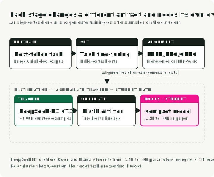
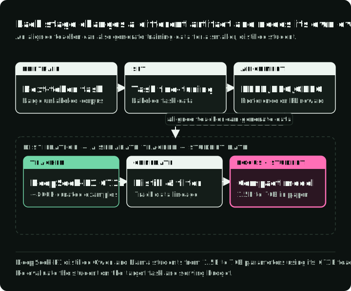
Pretraining is self-supervised next-token prediction on a large corpus. Its compute spans many orders of magnitude; Llama 3 405B, for example, used FLOPs. Supervised fine-tuning (SFT) adapts the pretrained model to task-specific labeled data. RLHF / RLAIF uses preference data to shape behavior: a conventional RLHF pipeline collects comparisons, trains a reward model, then optimizes the policy. RLAIF substitutes AI-generated feedback for some human judgments.
Compute depends on model size, sequence length, data volume, optimizer, and method. PPO also carries more model state than SFT because a typical setup includes policy, reference, reward, and critic models. I covered the full fine-tuning decision framework in LLM Fine-Tuning Guide.
24. LoRA and QLoRA: parameter-efficient fine-tuning
LoRA freezes the pretrained weights and injects trainable low-rank matrices () and () so that the updated weight is . The LoRA paper reduced GPT-3 175B to about 18 million trainable parameters in its setup. Rank is a tuning parameter rather than a task-complexity rule; select it with a quality and memory sweep. LoRA adapters can be merged into the base weights after training to avoid a separate adapter path at inference.
QLoRA loads the base model in 4-bit NF4 quantization while training LoRA adapters in BF16. NormalFloat4 places more quantization levels near zero, where weight density is highest. The paper fine-tuned a 65B model on a single 48 GB GPU and reported results close to its 16-bit baselines. Its runtime and memory trade-offs are specific to the tested stack.
25. Mixed-precision training
Every floating-point format allocates its bits across three fields: sign (always 1 bit), exponent (sets the dynamic range), and mantissa (sets the precision). More exponent bits mean a wider range of representable magnitudes; more mantissa bits mean finer distinctions between nearby values. Integer formats have no exponent at all and represent only evenly spaced whole numbers within a fixed range.
| Format | Bits | Layout (S / E / M) | Range | Precision | Common use |
|---|---|---|---|---|---|
| FP32 | 32 | 1 / 8 / 23 | ~7 decimal digits | Master weights, optimizer states (Adam momentum & variance) | |
| BF16 | 16 | 1 / 8 / 7 | ~2 decimal digits | Preferred training format; same range as FP32 and usually no loss scaling | |
| FP16 | 16 | 1 / 5 / 10 | ~3 decimal digits | Training with loss scaling (older GPUs); inference on pre-Hopper hardware | |
| FP8 E4M3 | 8 | 1 / 4 / 3 | ~1 decimal digit | Forward pass on Hopper (H100) — more precision for weights & activations | |
| FP8 E5M2 | 8 | 1 / 5 / 2 | ~0.6 decimal digits | Backward pass on Hopper — wider range for gradients | |
| INT8 | 8 | fixed-point | to | Exact integers | Post-training weight quantization for inference (W8A8); KV cache quantization |
| INT4 | 4 | fixed-point | to | Exact integers | Aggressive weight-only quantization (AWQ, GPTQ) for inference on memory-constrained hardware |
BF16 has the same range as FP32 because range is set by the exponent field, and BF16 keeps all 8 exponent bits from FP32. It gives up mantissa bits instead (7 vs 23), trading precision for a 2x memory reduction while avoiding many range problems that affect FP16 training. FP16 has only 5 exponent bits, capping its finite range at about 65K. Many gradients are instead too small for FP16 and underflow toward zero. Loss scaling multiplies the loss before backpropagation so those gradients remain representable, then unscales them before the optimizer step; dynamic scaling lowers the factor if overflow occurs. BF16’s wider exponent range usually avoids this requirement.
Integer formats are uncommon for the main training arithmetic because backpropagation needs a wide dynamic range. They are widely used for inference, where frozen weights can be mapped to calibrated scales. INT4 weight quantization cuts a 7B model from about 14 GB to 3.5 GB before runtime overhead; quality must be measured for the chosen model and method.
FP8 training on H100 via Transformer Engine uses E4M3 where precision matters and E5M2 where wider range matters. The FP8-LM paper reports that its mixed-precision framework trained GPT-175B 75% faster than its BF16 Megatron-LM baseline and 37% faster than NVIDIA Transformer Engine under the tested H100 setup. DeepSeek-V3 used FP8 mixed precision and reported about $5.6 million in rental-equivalent compute for its final training run, excluding R&D and infrastructure.
26. Gradient checkpointing
Each layer of the forward pass produces an intermediate output called an activation:
Normally all activations have to stay in memory because backpropagation needs them to compute gradients. For a deep transformer, the stored activations can take more memory than the model weights themselves.
Gradient checkpointing trades compute for memory by throwing most of those activations away and recomputing them on the fly during backprop. The standard strategy (Chen et al., 2016) divides a network of layers into evenly spaced segments and saves only the boundary activation of each segment. Those saved boundaries are the “checkpoints.” All intermediate activations within a segment are dropped immediately.
When the backward pass reaches a layer inside a segment, its activations are recomputed from the nearest checkpoint. For the evenly segmented strategy, saved activation memory drops from to . Actual memory savings and recomputation overhead depend on the model, checkpoint boundaries, sequence length, framework, and implementation, so measure both on the target training run. FlashAttention applies the same principle inside attention by not materializing the full attention matrix. Enable it in HuggingFace with gradient_checkpointing=True.
27. DeepSpeed ZeRO stages
In standard data parallelism, every GPU holds a complete copy of the model weights, gradients, and optimizer states. For Adam, each parameter takes 2 bytes for the FP16 weight + 4 bytes for the FP32 master weight + 4 bytes for momentum + 4 bytes for variance + 2 bytes for the gradient, which is 16 bytes per parameter. A 7.5B-parameter model needs ~120 GB per GPU, and every GPU stores the same thing. On 64 GPUs that is 64 identical 120 GB copies. A lot of waste.
DeepSpeed ZeRO (Zero Redundancy Optimizer) removes this duplication by sharding these components across GPUs instead of replicating them:
- Stage 1 — partition optimizer states. Each GPU stores only 1/N of the optimizer states (the FP32 master weights plus Adam’s first and second moments, 12 bytes/param). When a GPU needs to update a weight, it updates only its slice and broadcasts the result. Under the assumptions below, memory drops from ~120 GB to ~41.3 GB per GPU.
- Stage 2 — also partition gradients. Gradients (2 bytes/param) are no longer all-reduced to every GPU. Each GPU receives only the gradient slice it needs via reduce-scatter. Under the same assumptions, memory drops to ~28.1 GB per GPU.
- Stage 3 — also partition the model weights. Each GPU holds only 1/N of the FP16 weights. Before each layer’s forward or backward pass, the GPU calls all-gather to temporarily reconstruct the full layer weights from all other GPUs, computes, and discards the gathered weights. Under the same assumptions, memory drops to ~15.0 GB per GPU.
| Config | Optimizer States | Gradients | Weights | Approx. model-state memory per GPU (7.5B, 8 GPUs) |
|---|---|---|---|---|
| No ZeRO | Replicated | Replicated | Replicated | ~120 GB |
| Stage 1 | Partitioned | Replicated | Replicated | ~41.3 GB |
| Stage 2 | Partitioned | Partitioned | Replicated | ~28.1 GB |
| Stage 3 | Partitioned | Partitioned | Partitioned | ~15.0 GB |
These are approximate model-state values for a 7.5B-parameter model on 8 GPUs (world size ), with FP16 weights and gradients and FP32 Adam master weights, momentum, and variance. They exclude activations, temporary all-gather buffers, allocator fragmentation, and framework/runtime overhead. The calculation boundary is bytes per parameter, with each state divided by only when the table marks it as partitioned.
The tradeoff is communication. Stage 1 adds minimal overhead, and Stage 2 replaces all-reduce with reduce-scatter at similar cost. Stage 3 needs all-gather calls before every layer in both the forward and backward passes, roughly 1.5x communication volume versus standard data parallelism.
ZeRO-Infinity extends Stage 3 by offloading partitioned states to CPU RAM and even NVMe SSDs, which can make training models with trillions of parameters possible on limited GPU clusters. Storage offload adds PCIe and storage-transfer cost; its measured impact depends on the drive, PCIe topology, partitioning, prefetch, transfer overlap, and workload. Use it to satisfy capacity requirements rather than assuming a fixed slowdown, and profile the target configuration.
28. FSDP: PyTorch-native sharding
Fully Sharded Data Parallel (FSDP) is PyTorch’s built-in answer to DeepSpeed ZeRO-3. It shards parameters, gradients, and optimizer states across GPUs with the same core idea. The mechanics for each layer are a simple loop:
- All-gather the full parameters from all GPUs (temporarily reconstruct the complete layer).
- Compute the forward or backward pass for that layer.
- Free the gathered parameters immediately. Each GPU keeps only its own shard.
- Reduce-scatter gradients so each GPU gets only its assigned gradient slice.
Because FSDP is native to PyTorch, it integrates directly with PyTorch debugging tools, profilers, and torch.compile. Performance relative to DeepSpeed ZeRO-3 depends on wrapping policy, communication topology, offload settings, and model size, so compare them on the same cluster.
| Criteria | FSDP (PyTorch) | DeepSpeed ZeRO |
|---|---|---|
| Control style | Full sharding through PyTorch APIs | Selectable ZeRO stages |
| Offloading | CPU offloading | CPU + NVMe with ZeRO-Infinity |
| Framework integration | Native PyTorch, torch.compile paths | Separate library and config system |
| Selection test | Profile the target PyTorch workload | Profile required features and offload |
FSDP2 (2024–2025) is a rewrite that improves torch.compile integration for better kernel fusion, adds FP8 training support via TorchAO, and simplifies the API. Both FSDP and DeepSpeed are accessible through HuggingFace Accelerate, which lets you switch between them with a single config change.
29. Scaling laws and the Chinchilla trap
Chinchilla scaling (DeepMind, 2022) found a compute-optimal allocation near 20 training tokens per parameter under its assumptions. That objective does not include downstream serving cost. If a smaller model trained on more data reaches the required quality, it may cost less over a high-volume inference lifecycle.
One lifecycle-cost strategy is to train a smaller model on much more data:
| Model | Params | Training Tokens | Tokens/Param | Tokens/param ÷ 20 (derived) |
|---|---|---|---|---|
| Chinchilla | 70B | 1.4T | 20:1 | 1× |
| Llama 1 | 65B | 1.4T | 22:1 | 1× |
| Llama 2 | 70B | 2.0T | 29:1 | 1.4× |
| Llama 3 8B | 8B | 15T | 1,875:1 | 94× |
| Qwen3-0.6B | 0.6B | 36T | 60,000:1 | 3,000× |
This is the displayed tokens-per-parameter ratio divided by the Chinchilla paper’s approximate 20-token-per-parameter point. It is a descriptive ratio, not a measured quality or cost multiplier.
For a model served at high volume, spending more training compute on a smaller model can reduce lifecycle cost. Llama 3 8B illustrates the strategy, but whether it wins depends on the required quality and projected inference volume. “Chinchilla-optimal” refers to training-compute efficiency, which is a different objective from lifecycle cost.
30. RLHF, DPO, GRPO, and the alignment landscape
Alignment steers a pretrained model toward desired instructions, preferences, and safety policies. It does not by itself guarantee truthfulness or safe behavior. The methods below trade off implementation complexity, data requirements, exploration, and training stability.
The classic RLHF pipeline: SFT → collect human preference pairs → train a reward model on those pairs → fine-tune the policy with PPO (Proximal Policy Optimization). PPO holds 4 model copies in memory at once (policy, reference, critic/value model, reward model) and is hyperparameter-sensitive. It is also prone to reward hacking, where the model exploits quirks in the reward model, such as verbose, confident-sounding answers, instead of genuinely improving quality.
DPO (Direct Preference Optimization) skips the learned reward model and online RL loop by optimizing a loss on preference pairs directly. That simplifies the training pipeline. Standard DPO is offline: it trains on a fixed dataset and does not explore new responses during the update loop. Whether that limitation matters depends on the task and data coverage.
GRPO (Group Relative Policy Optimization, DeepSeek) removes PPO’s learned critic by generating multiple completions per prompt and using group-relative rewards as the baseline. This reduces the model-state burden relative to a typical PPO setup. Unlike DPO, GRPO is on-policy: the model generates fresh responses during training. DeepSeek-R1 combines GRPO with RLVR (reinforcement learning from verifiable rewards), using checks such as math answers, code compilation, and unit tests. These rewards are easier to audit than a learned preference score, but incomplete tests and proxy objectives can still be exploited.
| Method | Typical model state | Reward signal | Online/offline | Key limitation |
|---|---|---|---|---|
| PPO | 4 (policy, ref, critic, reward) | Learned reward model | Online | Reward hacking, complex tuning |
| DPO | 2 (policy, reference) | Implicit (preference pairs) | Offline | No exploration, fixed data |
| GRPO | 2 with rule rewards; 3 with learned reward (policy, reference, reward) | Explicit (rule/verifier or learned) | Online | Depends on reward quality and informative within-group variation |
31. Distillation: compressing knowledge across models
Knowledge distillation transfers capabilities from a large teacher to a smaller student. Logit-based distillation trains the student to match the teacher’s output distribution. Data-based distillation has the teacher generate examples that the student fine-tunes on. Data-based methods are common for LLMs because they can work across architectures and with API-only teachers, but their value is bounded by teacher quality, data coverage, filtering, and generation cost.
DeepSeek-R1 curated an approximately 800,000-example mixture—about 600,000 reasoning-related samples and 200,000 non-reasoning samples—and used it to distill Qwen2.5 and Llama 3 models from 1.5B to 70B parameters. In the paper’s evaluation:
- DeepSeek-R1-Distill-Qwen-32B scores 72.6% on AIME 2024 and 94.3% on MATH-500, above the paper’s reported OpenAI o1-mini numbers.
- DeepSeek-R1-Distill-Qwen-7B scores 55.5% on AIME 2024, above the paper’s QwQ-32B-Preview result with a smaller model.
In DeepSeek-R1’s small-model experiments, distillation outperformed direct GRPO on the tested base models. That result supports distillation for this setup; it does not establish a universal ranking between distillation and RL.
32. Synthetic-data generation
LLM-generated training data is used in several recurring patterns:
- Self-Instruct bootstraps from a small seed set of human-written instructions: the LLM generates new instructions, inputs, and outputs, which are filtered and added back to the pool. The Alpaca project used 52,000 examples generated from 175 seeds. Stanford reported data generation under 100, putting the initial reproduction cost under $600; its GPT-3.5 comparison was a limited project evaluation, not broad equivalence.
- Evol-Instruct (WizardLM) takes existing instructions and iteratively evolves them along complexity axes (adding constraints, deepening reasoning, making problems more concrete) to produce progressively harder training examples.
- Microsoft’s Phi-4 (14B) used synthetic data for much of pretraining, including generation, critique, self-revision, and instruction reversal. Its technical report compares the resulting STEM and coding performance with larger models on the selected benchmarks.
The risk that matters here is model collapse: when models are recursively trained on synthetic data from previous generations, the tails of the original distribution progressively vanish. The model overestimates common patterns and loses rare but important variations (Shumailov et al., 2024). A separate Ahrefs classifier study sampled one newly detected English page per domain from 900,000 pages in April 2025 and classified 74.2% as containing some AI-generated text. That vendor study is not a census of the web. Mitigation starts with blending synthetic and real data, filtering, and lineage tracking so recursively generated material can be measured.
Part VI — Scaling and deployment
Once a workload no longer fits or meets its SLO on one device, the choices are how to split work, which runtime exposes the needed controls, and whether every request needs the same model.
33. Four forms of parallelism
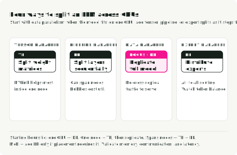
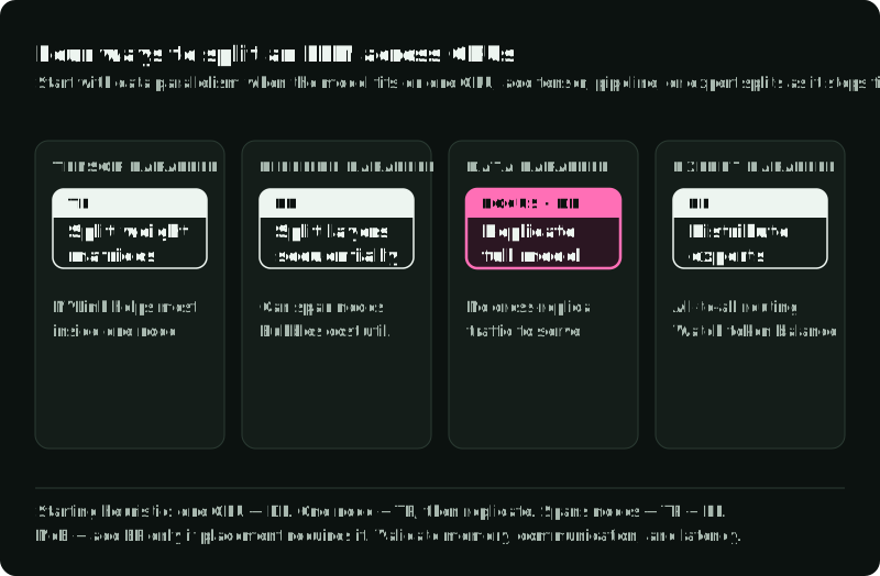
Tensor Parallelism (TP) splits individual weight matrices across GPUs and usually communicates after each layer. Fast intra-node links such as NVLink make it most practical within a node. More shards reduce per-device memory and compute but increase communication, so select the degree with a latency benchmark.
Pipeline Parallelism (PP) splits layers sequentially across GPUs, passing activations between stages. Its communication pattern can work across nodes, but pipeline bubbles and uneven stage times reduce utilization. Large deployments often combine TP within a node and PP across nodes.
Data Parallelism (DP) replicates the serving model so each replica handles independent requests without per-request cross-replica communication. It is efficient when the model fits and traffic can be balanced. In training, DP is commonly combined with ZeRO or FSDP to shard state.
Expert Parallelism (EP) distributes MoE experts across GPUs using all-to-all communication for token routing. Its performance depends on token balance, expert placement, and interconnect topology; all-to-all traffic can become the dominant bottleneck.
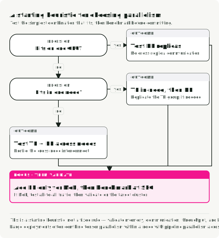
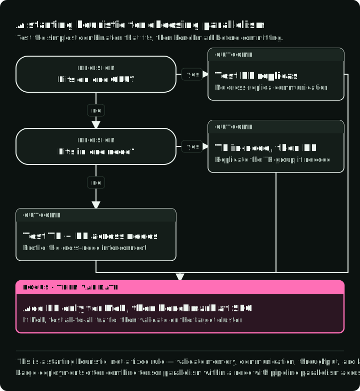
A starting parallelism heuristic:
- Model fits on one GPU: begin with independent replicas and measure DP scaling.
- Model fits within one node: test TP within the node, then replicate the group if traffic requires it.
- Model spans nodes: test a TP and PP combination against the interconnect and latency target.
- Mixture of experts: add EP only when expert placement requires it.
34. Serving frameworks compared
vLLM provides paged KV allocation, continuous batching, an OpenAI-compatible API, and several parallelism modes. Its model and hardware support changes frequently, so verify the target model against the current compatibility matrix.
SGLang combines RadixAttention for prefix reuse, a custom scheduler, and structured generation. Its published throughput gains depend on workload and configuration; compare it with vLLM and TensorRT-LLM using identical prompts, outputs, hardware, and SLOs.
TensorRT-LLM targets low single-request latency through CUDA graph fusion and kernel optimization, with native FP8/FP4 support. Its published numbers are hardware- and model-specific. The tradeoff is a steeper learning curve and NVIDIA-specific deployment surface.
TGI integrates with the Hugging Face ecosystem and supports several hardware backends. Check the repository’s current maintenance and feature status before selecting it for a new deployment.
Ollama emphasizes a simple local model workflow. Use it for development convenience; benchmark another serving stack when high concurrency or explicit SLO control matters.
llama.cpp is a portable C/C++ runtime with ARM, x86, Metal, CUDA, ROCm, and Vulkan paths. GGUF supports several quantization levels. Performance varies widely by model, quantization, context, and backend, so use its local benchmark tool for the target machine.
35. GPU selection for inference
The table compares published hardware characteristics. Vendor precision support does not make peak-compute figures directly comparable across formats, so select by memory fit first and benchmark the target workload. Check current cloud prices separately because they vary by provider, region, commitment, and availability.
| GPU | Memory | Bandwidth |
|---|---|---|
| B200 SXM | 180 GB HBM3e | Up to 8 TB/s |
| H200 SXM | 141 GB HBM3e | 4.8 TB/s |
| H100 SXM | 80 GB HBM3 | 3.35 TB/s |
| A100 80 GB SXM | 80 GB HBM2e | 2.039 TB/s |
Select first by memory fit, then by measured throughput at the latency target. H200’s 141 GB capacity can simplify some large-model deployments, while B200 adds FP4 support, 180 GB HBM3e, and a newer NVLink generation. Smaller GDDR-based GPUs can be economical for quantized models when their memory and interconnect limits match the workload.
AWQ and GPTQ serve 4-bit models by dequantizing supported matrix operations into a compute format such as FP16 or BF16. Compatibility and speed still depend on the model architecture, quantization format, serving backend, kernel, and GPU, so check the backend’s support matrix and benchmark the exact artifact. Hopper (H100/H200) and Ada (L40S/4090) natively accelerate FP8, and Blackwell (B200) adds native FP4 Tensor Cores. All listed GPUs support INT8 matrix operations.
LLM decode is often memory-bandwidth-bound, so HBM capacity and bandwidth can matter more than peak TFLOPS for serving workloads. Compare GPUs with the model, precision, batch distribution, context length, and latency target held constant.
36. Model cascading and routing
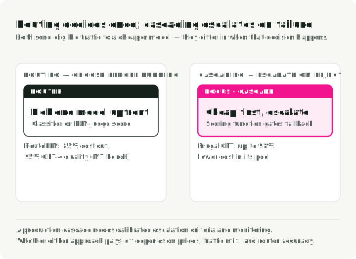
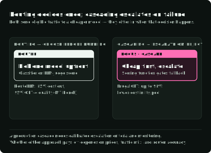
Model routing picks which LLM handles each query based on predicted complexity or capability. RouteLLM (LMSYS/UC Berkeley, ICLR 2025) reports an 85% cost reduction on its MT-Bench setup while retaining 95% of its GPT-4 quality baseline. Whether routing pays off depends on current prices, the traffic mix, router errors, and the quality floor.
Routers range from lightweight classifiers to LLM-based judges. Cascading is the sequential variant: a query starts with a cheaper model and escalates when a scoring function rejects the answer. FrugalGPT reports up to 98% lower cost or up to 4% higher accuracy in its evaluated model pool. A production cascade needs calibrated escalation criteria and monitoring for the queries the cheap model accepts incorrectly.
Part VII — Applications
Applications add their own failure surfaces. Retrieval can fail before generation begins, agents can choose an invalid action, and a prompt change can improve one task while breaking another.
37. Embedding models vs generative models
Embedding models encode text into fixed-dimensional vectors that capture semantic meaning. Unlike generative models that produce token sequences, they output one dense vector for the input, commonly with a few hundred to several thousand dimensions. Their backbones include bidirectional encoder-only transformers and decoder-derived models adapted for representation learning. A pooling layer often collapses per-token representations into one vector through mean pooling, a special classification token, or a model-specific last-token method. Contrastive fine-tuning then pushes semantically similar texts closer together and dissimilar texts farther apart.
Current embedding systems cover different deployment needs. Qwen3-Embedding-8B supports configurable output dimensions and many languages. Gemini Embedding 2 accepts text, images, video, audio, and documents. pplx-embed-v1-4B studies lower-precision dense embeddings. OpenAI text-embedding-3-large supports shortened embeddings through its dimensions parameter. These are examples, not a ranking: evaluate language, modality, task, dimension, and serving cost on one retrieval set.
Matryoshka Representation Learning (MRL, Kusupati et al., NeurIPS 2022) makes embedding dimensions flexible. Named after Russian nesting dolls, MRL structures an embedding so that its first dimensions are as informative as an independently trained -dimensional model. During training, MRL aggregates losses over a chosen set of prefix dimensions, usually consistent halvings; the paper’s 2048-dimensional example uses . The aggregated loss pushes the leading dimensions to carry coarse semantic information, with later dimensions adding finer detail.
After training, an MRL embedding can be truncated to a supported prefix dimension. OpenAI reports that text-embedding-3-large at 256 dimensions outperforms text-embedding-ada-002 at 1,536 dimensions on its cited MTEB comparison. That gives a 6x reduction in raw vector storage; search latency and database cost also depend on the index, metadata, filtering, and hardware.
The embedding model is one important component in a RAG pipeline, alongside parsing, chunking, search, reranking, and generation. If relevant evidence is not retrieved, a stronger generator cannot reliably recover it.
38. RAG architecture in production
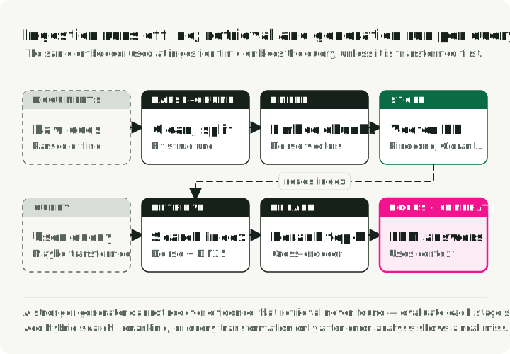
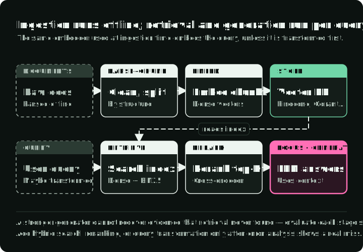
Retrieval-Augmented Generation supplies an LLM with documents retrieved at query time. It can provide current or private evidence that is absent from model weights, but retrieval does not guarantee that the answer uses that evidence correctly. A production RAG system is a multi-stage pipeline whose stages need separate evaluation.
The ingestion pipeline runs offline. Raw documents (PDFs, HTML, Markdown, databases) are first parsed into clean text, which is harder than it sounds: PDF parsing alone can lose tables, headers, and formatting. The text is then split into chunks, which are embedded and indexed independently.
Chunking affects both retrieval recall and the context available to the generator. Useful sizes depend on document structure, query granularity, embedder limits, and reranker limits. Common approaches are fixed-size with overlap, recursive splitting along document boundaries, and semantic chunking by embedding similarity. Compare them on page- or section-level relevance labels instead of adopting one token range universally.
Each chunk is then embedded with a model like those in Section 37 and stored in a vector database (Pinecone, Weaviate, Qdrant, pgvector, and so on).
The retrieval pipeline runs at query time. Start with a measurable baseline, then add stages when error analysis shows they address a real miss:
- Hybrid search combines dense vector retrieval with sparse retrieval such as BM25, often merged through Reciprocal Rank Fusion (RRF). Dense search handles semantic paraphrases; sparse search catches exact identifiers, error codes, and acronyms. Vendor benchmarks report gains over vector-only baselines, but the size depends on the corpus and relevance labels.
- Reranking passes retrieved candidates through a model that scores the query and document together. This can improve fine-grained relevance at the cost of another model call. Candidate count, retained count, and latency should be tuned together. I covered the full multi-stage pipeline in Building a Modern Search Ranking Stack.
- Query transformation rewrites the user’s query before retrieval to improve recall. HyDE (Hypothetical Document Embeddings) has the LLM generate a hypothetical answer, which is then embedded and used for retrieval. Multi-query expansion generates multiple phrasings of the same question. Step-back prompting asks a more general question first to pull in broader context.
The common failure modes:
- Retrieval failure — the correct document exists but is not retrieved. Test chunking, query transformation, hybrid search, and metadata filtering against the miss.
- Context poisoning — irrelevant retrieved chunks mislead the LLM. Test reranking, context filters, and smaller retained sets.
- Lost-in-the-middle — in the tested multi-document question-answering and key-value retrieval settings, Liu et al. found answer performance was generally highest when relevant information appeared near the beginning or end of the input and lower when it appeared in the middle.
GraphRAG (Microsoft, 2024) augments vector retrieval with an extracted entity and relationship graph. It targets corpus-level and relationship-heavy questions that flat chunk retrieval may miss. The trade-off is additional extraction, indexing, storage, and evaluation work.
Practitioner guides publish latency ranges for embedding, search, reranking, and generation, but those figures vary by region, corpus, hardware, and model. Measure each stage in traces and evaluate the quality change before accepting the added latency.
39. Agent architectures and tool calling
LLM agents use models to select and sequence tool calls around an evolving state. Three useful orchestration patterns are:
- ReAct — interleaves action selection with observations. It can adapt after each tool result, but a growing history raises token and latency cost.
- ReWOO — plans tool calls with placeholders, executes independent work in parallel, and then synthesizes. Its paper reports token savings over ReAct, but the fixed plan needs an explicit recovery path when a tool fails.
- Planner-executor — separates planning from execution and can add a re-planning policy after failure. It permits model specialization but adds orchestration state and another decision boundary.
| Pattern | Token tendency | Adaptability | Useful starting point |
|---|---|---|---|
| ReAct | Higher | Updates after observations | Uncertain or exploratory tool use |
| ReWOO | Lower | Fixed plan unless extended | Predictable work with parallel steps |
| Planner-executor | Medium | Can revise the explicit plan | Longer tasks that benefit from control |
Function calling is a common mechanism for tool invocation. APIs expose tool definitions and return structured arguments, reducing the need to parse free-form text. Schema-valid arguments can still select the wrong tool or contain invalid values. Parallel function calling can reduce round trips when operations are independent.
Structured output and constrained decoding enforce a schema by restricting the tokens available at each generation step. Engines such as xgrammar, used in vLLM and SGLang, can remove many syntax and parsing failures with low overhead in supported configurations. They do not guarantee that the extracted values or decisions are correct. Schema-Guided Reasoning (SGR) uses field order and schema structure to make intermediate state inspectable before the final decision. Its three patterns are Cascade (sequential steps), Routing (union types as semantic switches), and Cycle (bounded lists).
Tool-selection quality, end-to-end latency, and token cost usually worsen as the tool set and action depth grow. Measure those curves with the actual tool descriptions and failure distribution. Frameworks such as LangGraph can make state and recovery paths explicit, but they do not remove the evaluation burden.
40. Prompt engineering for production
Production prompting is an evaluation problem: change one part of the prompt or context, then measure task quality and failure modes. The techniques below are common starting points, not a universal order.
Few-shot examples are often effective for controlling output format. Start with 3–5 examples that cover empty inputs, ambiguous queries, and multi-part answers, then measure the result on a held-out set. Examples should span the real input distribution rather than only the happy path. More examples consume context and do not guarantee further gains.
Chain-of-thought (CoT) prompting asks a model to expose intermediate reasoning before answering. Kojima et al. reported gains from the suffix “Let’s think step by step” on their tested reasoning tasks, but the effect varies by model and newer reasoning APIs may not expose hidden traces. For production, prefer an inspectable task decomposition or concise rationale when it is useful to the evaluator. Self-consistency (Wang et al., 2023) samples several reasoning paths and aggregates the answers, trading extra inference cost for robustness on suitable tasks.
Structured output with explicit JSON schemas (Section 39) removes many parsing failures. Constrained decoding engines such as xgrammar can enforce the supported grammar during generation; factual accuracy and semantic validity still require evaluation, and unsupported schema features may still need handling.
Prompt chaining breaks a task into focused stages, for example classify intent → retrieve context → generate response → validate output. It can localize failures, allow different models per stage, and expose cacheable intermediate state. It also adds interfaces and latency, so compare it with a single-call baseline.
Temperature changes the sampling distribution. Low values are a reasonable starting point for classification or extraction; higher values can increase diversity for ideation. Exact behavior differs across model APIs and interacts with top_p, top_k, and provider defaults, so sweep the supported settings on the task rather than copying one range.
System vs user message separation keeps persistent policy apart from per-request content. Chat templates and instruction tuning give these roles different priority, but they do not make a system message an enforcement boundary. Put stable behavior in the system message, keep untrusted data in user or tool content, and enforce hard constraints such as PII removal outside the model as well.
Context engineering expands prompt work to the assembly of retrieved documents, tool results, conversation history, and examples. Liu et al. found a lost-in-the-middle effect in the long-context models they tested, so position should be part of the evaluation rather than assumed irrelevant. I covered the broader workflow in Context Engineering for AI Agents.
Part VIII — Production operations
Production operations turns the earlier concepts into admission limits, load tests, alerts, and capacity decisions under real traffic.
41. Rate limiting for variable-cost requests
Traditional requests-per-second rate limiting assumes roughly equal cost per request. LLMs break that assumption. A 10-token classification prompt and a 100K-token document analysis hit the same API endpoint but differ in cost by four orders of magnitude. Rate-limiting by RPS either lets expensive requests through unchecked or starves cheap requests unnecessarily.
Production systems need token-based rate limiting across multiple dimensions. OpenAI documents request and token limits by usage tier. Anthropic separates input-token and output-token limits. Exact quotas and algorithms can change, so treat the provider documentation as the source of truth; the architectural point is to budget requests and tokens independently.
The practical implementation pattern is a multi-dimensional limit hierarchy (user → application → organization → global), with priority tiers for premium access. At the request level, the technique that matters is token budget reservation: estimate total tokens (input + max_tokens) at admission time, deduct from the bucket, then adjust when the request completes with actual usage. That prevents a burst of long-generation requests from exhausting capacity before they even start producing output.
For self-hosted deployments, the equivalent is provisioned throughput: reserving dedicated GPU capacity for target token rates. For vLLM deployments, that means configuring admission control around active decode slots and KV cache pressure rather than request count alone. As Section 5 explains, throughput and admission both need token-aware limits.
42. Failure modes to design against
LLM serving adds failure modes tied to variable sequence length, KV memory, and long-running decode work. Design and load-test the defenses before production traffic depends on them.
Out-of-Memory (OOM) is a common failure. A 70B FP16 model needs about 140 GB for weights alone, and KV cache for a single Llama 3.1 70B 128K-context sequence can add about 40 GB under the assumptions in Section 6. The gap between “fits in memory” and “OOM under load” is smaller than it looks because a batch of long-context requests can consume more KV memory than expected. Prevention combines a measured memory reserve with quantization and paged KV allocation. For workloads with high KV pressure, LMCache can offload KV data to CPU memory or disk; use its published results as a starting point and benchmark the local memory hierarchy.
Preemption happens when KV cache pressure forces the scheduler to evict or recompute work. The exact strategy depends on the serving version and configuration. From the user’s side, the symptom is higher end-to-end latency without an obvious application error. Watch preemption counts and correlate them with KV use, queue depth, and request lengths.
Tail latency can spike when large prefills delay decode work. Chunked prefill (Section 7) and length-aware scheduling target this interference. The Learning-to-Rank scheduler and CascadeInfer papers report improvements over their baselines under their evaluated workloads, but the exact result depends on the request-length distribution and scheduler configuration.
Cascading failures can start when slow requests grow the queue, upstream clients time out, and retries add more load. Defenses include admission control, per-tenant concurrency limits, output caps, retry budgets, and gateway circuit breakers. Disaggregated prefill and decode pools may help when load tests show persistent phase interference.
43. Monitoring LLM systems
LLM monitoring is different from traditional API monitoring in some basic ways. Every request has variable cost, two distinct phases with different bottlenecks, and a memory footprint that depends on both input length and generation length. Standard metrics like request latency and error rate miss most of what matters.
Goodput is the number of requests per second that meet all defined SLO thresholds, such as TTFT, TPOT, and total latency. It is a useful combined measure because raw throughput can look healthy while latency SLOs fail: a system processing 100 requests per second but missing its thresholds on 40% of them has a goodput of 60 requests per second. Optimizing for goodput keeps the performance distribution visible instead of reporting only the mean.
vLLM exposes a Prometheus endpoint at /metrics with running and waiting requests, KV cache use, generation-length distributions, and prefix-cache statistics. Metric names can change across releases, so bind dashboards to the deployed version. A typical stack uses Prometheus for metrics, Grafana for visualization, and OpenTelemetry-compatible traces across application and serving components.
Useful alert patterns include the following. Derive their thresholds from load tests rather than copying these examples unchanged:
- Preemption count spikes — the runtime is swapping or recomputing work, which adds latency without an application error.
- KV cache utilization approaching the tested preemption region — add capacity or shed load before evictions cascade.
- Queue depth persistently above the tested batch envelope — admission control should start rejecting or deprioritizing.
- TTFT rising while TPOT stays flat — this divergence points first to queuing, admission, network, or prefill pressure rather than decode throughput. Use traces and queue metrics to distinguish among them.
44. Cost optimization: a compounding strategy
Provider prices and input-to-output price ratios change. Pull current rates before a purchasing decision; model tier and output length can dominate the bill even before infrastructure optimizations.
Several approaches can be stacked, but only after measuring which ones apply to the workload:
- Quantization from FP16 to INT4 cuts weight memory by 75%. Whether that reduces the bill depends on kernel speed, batch size, and hardware utilization (Section 9).
- Model routing sends eligible traffic to cheaper models. Measure the router’s false-accept rate and end-to-end quality before increasing the share handled by the cheaper model (Section 36).
- Prompt caching reduces repeated-prefix work. Provider discounts and rate-limit treatment change over time, so combine measured hit rate with current terms (Section 16).
- Batch APIs can discount non-real-time work such as evaluations, synthetic-data generation, and bulk classification. Check current prices and completion windows.
- Self-hosting can win at sustained utilization, but there is no universal token-volume break-even. Include engineering, orchestration, observability, capacity slack, and on-call costs in addition to GPU rental.
Multiplying the illustrative factors gives a large theoretical reduction, but the inputs are not independent: quantization changes throughput, routing changes quality mix, and caching and batching apply only to eligible traffic. Build the estimate from measured traffic shares and validate it against the invoice.
45. Capacity planning and autoscaling
Capacity planning for LLM serving must account for variable request cost, long-running decode work, and sequence-dependent memory. Depending on the workload, the limiting resource may be KV memory, memory bandwidth, compute, or the interconnect.
The theoretical memory ceiling on concurrent requests comes from the KV-cache budget:
For capacity arithmetic, suppose the runtime exposes a 40 GiB KV budget for Llama 3.1 70B with an FP16 KV cache. Each 4K sequence uses about 1.25 GiB and each 128K sequence about 40 GiB. That budget therefore fits at most about 32 4K sequences or one 128K sequence before allocator, runtime, workload-variance, and SLO overhead. This is why GPU selection and KV cache optimization directly drive the capacity plan.
The capacity formula for fleet sizing:
Convert both rates to the same time unit before dividing. The detail that matters is “at target SLO.” A safety-factor multiplier such as 1.3 reserves 30% headroom; choose it from measured burstiness, failures, and recovery time. Peak token throughput and SLO-compliant throughput can differ sharply as concurrency rises. Benchmark with the real prompt and output-length distribution at the required TTFT and TPOT thresholds rather than using a theoretical maximum.
GPU utilization is insufficient as the only autoscaling signal because it can stay high during both healthy processing and overload. Combine it with queue depth, KV cache utilization, and goodput degradation. Tune thresholds from load tests; values such as 80% KV utilization are starting points, not universal limits. These metrics are introduced in Section 43.
Scale-to-zero can fit development and staging environments with long idle periods. Serverless inference platforms and Kubernetes-based autoscalers such as KEDA can remove idle capacity, but the savings and cold-start time depend on model size, image and weight caching, and infrastructure. Measure startup time before using the same policy for latency-sensitive production traffic.
Use the guide to choose the next measurement
The concepts interact, but they still produce a small set of useful first measurements. KV-cache demand constrains batch size alongside weight memory, runtime overhead, and request lengths. Larger batches can raise arithmetic intensity, while continuous batching increases KV-allocation churn and PagedAttention reduces the resulting fragmentation.

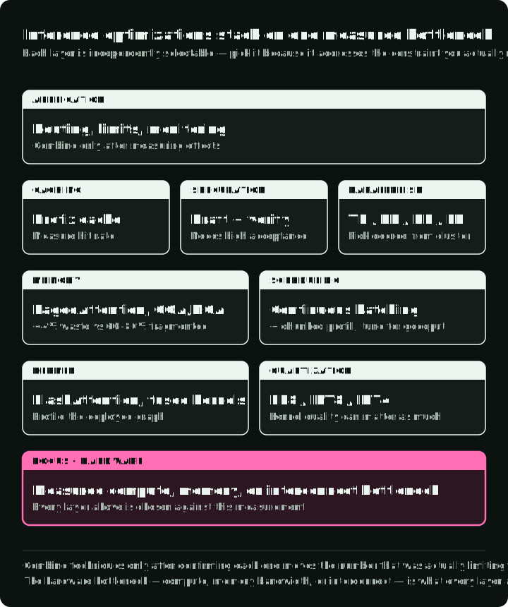
On the training side, lifecycle cost can favor training a smaller model on more tokens, as Llama 3 8B illustrates. GRPO reduces the critic-state burden of PPO. In DeepSeek-R1’s tested small-model setup, distillation outperformed direct RL. These are options to evaluate, not a recipe.
| Symptom or decision | Start with | Measure before changing the stack |
|---|---|---|
| First token is slow | Prefill and decode, TTFT | Queue time, prompt length, prefill time, and P99 TTFT |
| Tokens stream slowly | Roofline, TPOT | TPOT by concurrency, memory bandwidth, and batch shape |
| Long contexts trigger preemption or OOM | KV cache, PagedAttention | KV use, request lengths, allocator waste, and preemption count |
| A model does not fit the budget | Quantization, GPU selection | Quality, kernel throughput, memory reserve, and target-SLO goodput |
| A training run does not fit | LoRA and QLoRA, ZeRO, FSDP | Model-state memory, communication, throughput, and held-out quality |
| Cost is rising | Routing, cost optimization | Traffic eligibility, quality errors, cache hit rate, and invoice data |
Routing, caching, quantization, and hardware choice compound only when each is evaluated against the same quality and latency target. Pick one symptom, establish that baseline, and make the next change easy to reverse.
Further reading
Related deep-dives from this blog, organized by topic:
- LLM Fine-Tuning Guide — when to fine-tune vs. RAG vs. prompt engineering
- Open-Source LLM Variants and File Formats — matching model variants and quantized formats to hardware
- LoRAX Serving Guide — serving thousands of LoRA adapters in production
- Scaling Large Language Models — multi-GPU and multi-node strategies
- Local LLMs on macOS — hands-on setup with llama.cpp and Ollama
- AI Agent Reasoning Loops in 2026 — deep dive into ReAct, ReWOO, and planner-executor loops
- AI Agent Memory Architecture in 2026 — checkpoints, vector stores, and document memory for stateful agents
References
Organized by topic area.
Inference and attention
- FlashAttention: Fast and Memory-Efficient Exact Attention with IO-Awareness - Dao et al., NeurIPS 2022
- FlashAttention-2: Faster Attention with Better Parallelism and Work Partitioning - Dao, 2023
- FlashAttention-3: Fast and Accurate Attention with Asynchrony and Low-precision - Shah et al., NeurIPS 2024
- Flash-Decoding for long-context inference - Dao et al., 2023
- Efficient Memory Management for Large Language Model Serving with PagedAttention - Kwon et al., SOSP 2023
- Orca: A Distributed Serving System for Transformer-Based Generative Models - Yu et al., OSDI 2022
- GQA: Training Generalized Multi-Query Attention - Ainslie et al., 2023
- Triton: an intermediate language and compiler for neural network computations - Tillet et al., MAPL 2019
- FlashNorm: Fast Normalization for LLMs - 2024
- Deep Kernel Fusion for Transformers - DeepFusionKernel, 2026
Speculative decoding
- Accelerating Large Language Model Decoding with Speculative Sampling - Chen et al., 2023
- EAGLE-3: Scaling up Inference Acceleration of Large Language Models - Li et al., NeurIPS 2025
- Medusa: Simple LLM Inference Acceleration Framework with Multiple Decoding Heads - ICML 2024
Quantization
- AWQ: Activation-aware Weight Quantization for LLM Compression and Acceleration - MLSys 2024 Best Paper
- GPTQ: Accurate Post-Training Quantization for Generative Pre-trained Transformers - Frantar et al., ICLR 2023
- Marlin: Mixed-Precision (FP16xINT4) LLM Inference Kernel - Frantar et al., 2024
Training and fine-tuning
- LoRA: Low-Rank Adaptation of Large Language Models - Hu et al., ICLR 2022
- QLoRA: Efficient Finetuning of Quantized LLMs - Dettmers et al., NeurIPS 2023
- ZeRO: Memory Optimizations Toward Training Trillion Parameter Models - Rajbhandari et al., SC20
- ZeRO-Infinity: Breaking the GPU Memory Wall for Extreme Scale Deep Learning - Rajbhandari et al., 2021
- Self-Instruct: Aligning Language Models with Self-Generated Instructions - Wang et al., ACL 2023
- WizardLM: Empowering Large Language Models to Follow Complex Instructions - Xu et al., ICLR 2024
- Phi-4 Technical Report - Microsoft, 2024
- AI models collapse when trained on recursively generated data - Shumailov et al., Nature 2024
Alignment
- Direct Preference Optimization: Your Language Model is Secretly a Reward Model - Rafailov et al., NeurIPS 2023
- DeepSeekMath: Pushing the Limits of Mathematical Reasoning in Open Language Models - Introduced GRPO
- DeepSeek-R1: Incentivizing Reasoning Capability in LLMs via Reinforcement Learning - DeepSeek, 2025
Scaling and architecture
- The Llama 3 Herd of Models - Meta, 2024
- LLaMA: Open and Efficient Foundation Language Models - Touvron et al. (Meta), 2023
- Llama 2: Open Foundation and Fine-Tuned Chat Models - Touvron et al. (Meta), 2023
- Qwen3 Technical Report - Qwen Team (Alibaba), 2025
- Training Compute-Optimal Large Language Models - Hoffmann et al. (Chinchilla), NeurIPS 2022
- RoFormer: Enhanced Transformer with Rotary Position Embedding - Su et al., 2021
- YaRN: Efficient Context Window Extension of Large Language Models - Peng et al., ICLR 2024
- SGLang: Efficient Execution of Structured Language Model Programs - Zheng et al., NeurIPS 2024
- Mixtral of Experts - Jiang et al. (Mistral AI), 2024
Embeddings
- Matryoshka Representation Learning - Kusupati et al., NeurIPS 2022
- pplx-embed-v1: Diffusion-Pretrained Dense and Contextual Embeddings - Perplexity AI, 2026
Agent architectures
- ReAct: Synergizing Reasoning and Acting in Language Models - Yao et al., ICLR 2023
- ReWOO: Decoupling Reasoning from Observations for Efficient Augmented Language Models - Xu et al., 2023
Routing
- RouteLLM: Learning to Route LLMs with Preference Data - Ong et al., ICLR 2025
Benchmarks
- MLPerf Inference v5.0 Results - MLCommons, April 2025
Serving architectures
- Taming Throughput-Latency Tradeoff in LLM Inference with Sarathi-Serve - Agrawal et al., OSDI 2024 (Chunked prefill)
- Splitwise: Efficient Generative LLM Inference Using Phase Splitting - Patel et al., ISCA 2024 (Disaggregated Serving)
- DistServe: Disaggregating Prefill and Decoding for Goodput-optimized Large Language Model Serving - Zhong et al., OSDI 2024 (Disaggregated Serving)
Serving frameworks
- vLLM - PagedAttention-based serving engine
- SGLang - RadixAttention and structured generation
- TensorRT-LLM - NVIDIA optimized inference
- llama.cpp - Portable C/C++ inference
- DeepSpeed - Microsoft distributed training library
- Ollama - Local LLM runner
Operations
- Efficient LLM Scheduling by Learning to Rank - Fu et al., NeurIPS 2024 (vLLM-LTR)
- CascadeInfer: Length-Aware Scheduling of LLM Serving with Low Latency and Load Balancing - Yuan et al., 2025
- Goodput metric as measure of ML productivity - Google Cloud, 2024
- vLLM Optimization and Tuning - vLLM Documentation
- vLLM Metrics - vLLM Documentation
- LMCache: KV Cache Management for LLM Serving - KV cache offloading
- OpenAI Rate Limits - OpenAI API Documentation
- Anthropic Rate Limits - Anthropic API Documentation