DeepSeek mHC: Manifold-Constrained Hyper-Connections

Modern deep learning rests on the residual connection. Hyper-Connections (HC) explore another architectural dimension: widen the residual state into several interacting streams. DeepSeek’s Manifold-Constrained Hyper-Connections (mHC) paper studies how to keep that routing stable at larger training scales.
This post starts with standard residual connections, then adds Hyper-Connections and the instability they create. The mHC constraint and its implementation cost come at the end.
Why residual connections work
The depth problem
Adding layers can increase capacity, but it also makes optimization and signal propagation harder. Depending on initialization, normalization, and architecture, forward activations or backward gradients can shrink, grow, or become poorly conditioned across depth.
The residual solution
The ResNet paper introduced a simple fix. Instead of learning a direct mapping, learn the residual, the difference from identity:
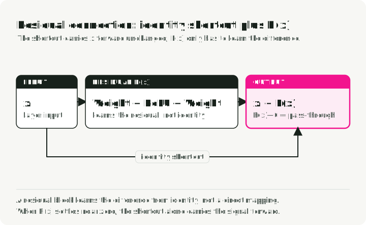
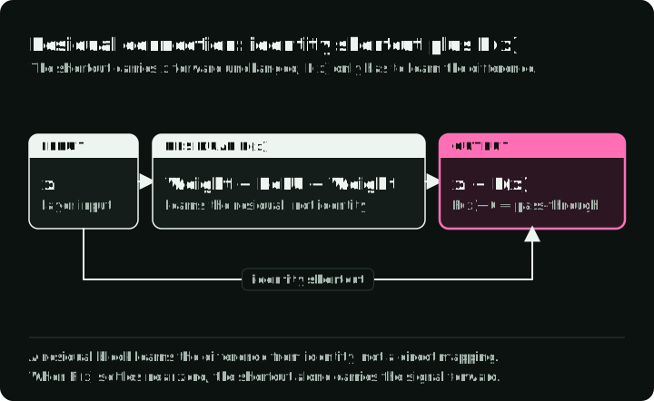
The useful property is the identity shortcut. When the residual function outputs zero, the layer becomes a pass-through. Two consequences follow:
- A direct gradient term: backpropagation includes a path through the identity component.
- A simple fallback mapping: the residual branch can stay near zero when a layer does not need to change the state much.
This does not eliminate every optimization problem, but it made substantially deeper networks practical.
How layer normalization changes the residual path
Transformers added a new variable: where to put Layer Normalization (LN). The decision looks minor and isn’t.
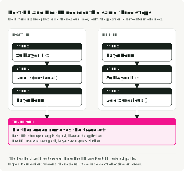
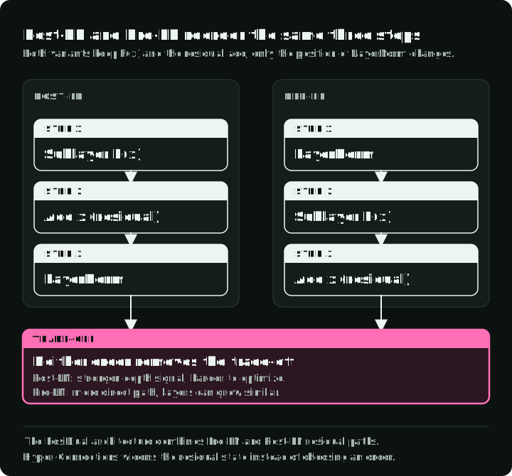
| Variant | LN Placement | Advantage | Key Limitation |
|---|---|---|---|
| Post-LN | After residual block | Strong depth contribution | Can be harder to optimize at depth |
| Pre-LN | Before residual block | More direct residual path | Adjacent-layer representations can become increasingly similar |
The ResiDual architecture combines Pre-LN and Post-LN residual paths. HC widens the residual state instead.
Hyper-Connections add parallel residual streams
Hyper-Connections (HC) expands the residual stream’s width rather than adding depth.
What a stream means
In a standard Transformer, each token has a -dimensional state that passes through the blocks. At the start of the network, HC replicates that input embedding times, where is the “expansion rate”, typically 4. The -dimensional hidden state becomes an “hyper hidden matrix”.
In Hyper-Connections, a stream is one of those parallel instantiations of the state.
The copies begin identically, then diverge as learned maps read from, write to, and mix the streams. The paper interprets them as multiple connection patterns across depth; it does not require each stream to acquire a fixed human-readable role.
Core mechanisms
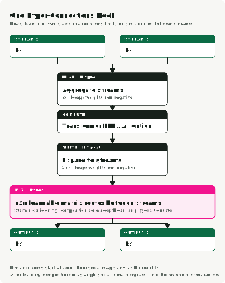
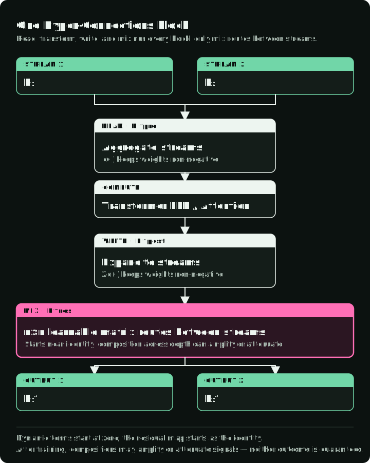
Instead of one residual pathway, HC keeps parallel streams flowing through the entire network. At each transformer block, three operations run, each controlled by small learnable weights:
- Read (): aggregate the streams into the -dimensional input consumed by the attention or feed-forward block.
- Write (): map that block’s output back into updates for the streams.
- Mix (): apply an residual map before adding the block update.
These maps can be static parameters plus input-dependent terms. The residual map is the stability-critical part because it is multiplied repeatedly across depth.
What the HC paper reports
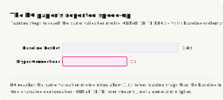
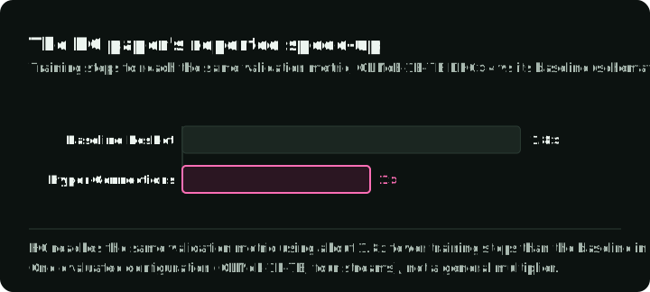
The HC paper reports 1.8× faster convergence for its OLMoE-1B-7B DHC×4 configuration relative to its baseline, plus downstream gains at 500B tokens (Section 1). That is one evaluated configuration, not a general speed multiplier for four streams.
The scaling problem
The mHC paper reports instability when it scales unconstrained HC to its 27B setup.
Why unconstrained HC can become unstable
The same unconstrained maps that make HC flexible also remove the guaranteed identity path that makes residuals easy to train.
The composite-map problem
In standard residuals:
When , this is identity: . Signal passes through unchanged.
In Hyper-Connections, the residual path includes a matrix multiplication:
Over L layers, the signal becomes:
The behavior depends on the composite matrix, not on whether individual entries sit above or below 1. If successive maps have operator gains above one along an aligned direction, signals can grow; gains below one can attenuate them. Negative entries can also introduce cancellation.
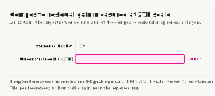
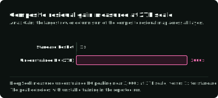
The mHC paper measures that gain with Amax Gain Magnitude: the maximum absolute row sum for forward propagation and column sum for backward propagation in a composite residual map. In its 27B HC experiment, the peak approaches 3,000 and coincides with unstable training behavior (Section 5.4).
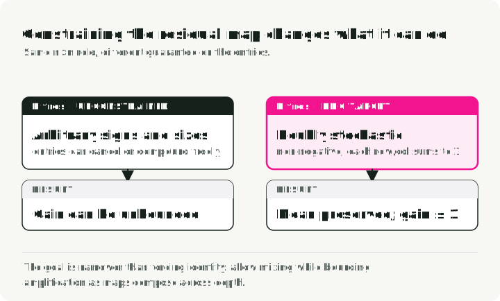
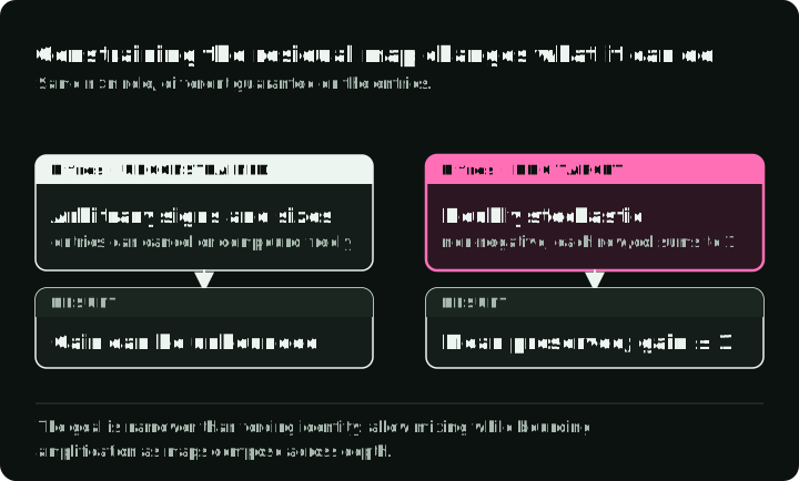
The design goal is therefore narrower than forcing every map to be the identity: allow inter-stream mixing while bounding amplification across compositions.
The mHC constraint
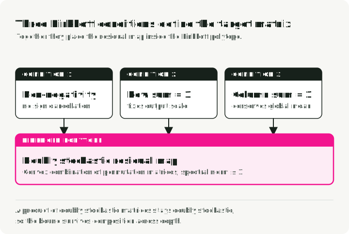
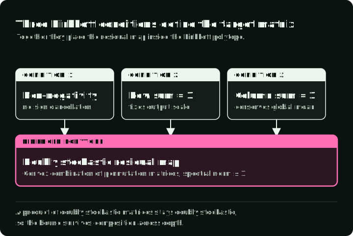
mHC keeps inter-stream routing but constrains each residual mixing matrix to the Birkhoff polytope, the set of doubly stochastic matrices. Such a matrix has non-negative entries, and each of its rows and columns sums to one. The constraint makes each output stream a convex combination of input streams and bounds the residual map’s spectral norm by one.
What double stochasticity guarantees
Double stochasticity buys three properties at once:
| Constraint | Consequence |
|---|---|
| Non-negativity | Each output is a convex combination, without sign cancellation |
| Row sum = 1 | A constant signal across streams remains constant |
| Column sum = 1 | The global mean across streams is conserved |
This is not literal Euclidean-energy conservation. A doubly stochastic map can smooth differences between streams. It provides mean conservation and non-expansive routing under the stated norm bound.
The constraint has three further consequences:
- Spectral norm ≤ 1: the residual routing map cannot amplify the Euclidean norm.
- Closed under multiplication: a product of doubly stochastic matrices remains doubly stochastic, so the constraint survives composition across depth.
- Convex mixing: by the Birkhoff-von Neumann theorem, the map lies in the convex hull of permutation matrices.
Sinkhorn-Knopp projection
The learnable residual logits are unconstrained. mHC first exponentiates them to obtain a positive matrix, then alternates column and row normalization. With enough iterations, this Sinkhorn-Knopp process approaches a doubly stochastic matrix; the paper uses 20 iterations as a practical, approximate differentiable projection rather than an exact constraint.
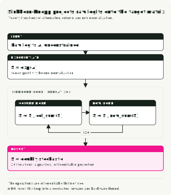
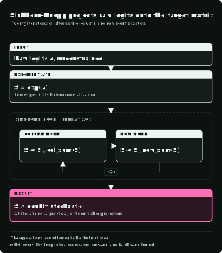
For raw logits , the procedure is:
S = exp(A)
repeat 20 times:
    S = S / column_sum(S)
    S = S / row_sum(S)
return S
The operations are differentiable, but they are not free. mHC relies on a fused forward kernel and a custom backward kernel that recomputes the intermediate normalization states on chip.
Parameterization details
- Residual map: exponentiation plus Sinkhorn normalization produces the approximately doubly stochastic .
- Read and write maps: and . Both maps remain non-negative, reducing cancellation from mixed-sign coefficients (Section 4.2).
Complete mHC architecture
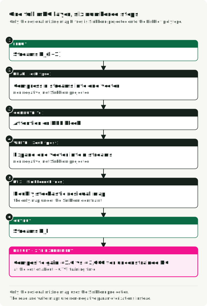
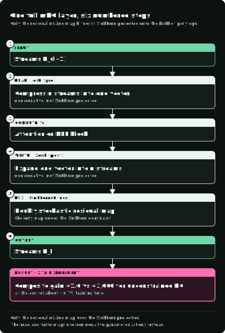
The flow through each block:
- Input: parallel residual streams enter the layer.
- Read (): the streams combine into the input consumed by the layer function. The paper uses , which makes the coefficients non-negative.
- Computation: the standard Transformer block (Attention or MLP) processes the single aggregated vector.
- Write (): the block output is mapped into updates for the streams with . The coefficients remain non-negative.
- Mix (): the approximately doubly stochastic residual map mixes the incoming streams before the update is added.
- Output: the updated stream matrix moves to the next layer.
Only the residual mixing map uses the Sinkhorn projection. The read and write maps use non-negative parameterizations. That distinction matters because the paper’s composition guarantee applies to .
Infrastructure required for the reported overhead
Four streams increase residual-state memory access, activation storage, and pipeline communication. The paper’s 6.7% timing result depends on the following co-designed implementation.
Kernel fusion
The implementation fuses operations that share memory access, uses mixed precision where appropriate, and implements most custom kernels with TileLang. The Sinkhorn loop and its custom backward pass run inside dedicated kernels to reduce memory traffic and launch overhead.
Selective recomputation
Storing every intermediate Sinkhorn state for backpropagation would blow up memory. Instead, mHC:
- Frees intermediate activations after the forward pass.
- Recomputes them on-the-fly during the backward pass.
An extended DualPipe schedule overlaps parts of communication, recomputation, and layer work at pipeline boundaries. The achieved overlap is specific to this training system.
Reported system result
For the paper’s large-scale setup, expansion rate adds 6.7% training time relative to its baseline (Section 4.3). This is a system result, not the overhead of a plain framework implementation.
What the experiments establish
In the 27B comparison, unconstrained HC reaches a peak composite Amax Gain near 3,000. With 20-step approximate Sinkhorn projection, mHC’s composite backward gain deviates from one but remains bounded at roughly 1.6 in the reported analysis (Section 5.4).
The authors also train 3B, 9B, and 27B DeepSeek-V3-inspired MoE variants (Section 5.3). At 27B, mHC beats the standard residual baseline on all eight reported downstream benchmarks, and beats HC on six of eight (Table 4). HC is slightly higher on GSM8K and MATH. These are in-house pretraining experiments from the proposing team, so independent replication and comparisons on other architectures remain open.
Trade-offs and open questions
mHC is not a drop-in win for every model. Four questions remain:
- System overhead: 6.7% is the optimized paper result; another runtime, device topology, or model shape may see a different cost.
- Implementation complexity: a reference implementation can express the method, but matching the reported throughput requires custom kernels, recomputation, and schedule changes.
- Mixing bias: double stochasticity preserves the cross-stream mean and prevents expansion through , but it can smooth differences between streams. The block update still changes the overall representation.
- Evidence scope: the strongest evidence is language-model pretraining on DeepSeek-V3-inspired MoE architectures. Generalization to other model families is not yet established by this paper.
Key takeaways
- Residual connections work because of identity mapping: the ability to pass signals through unchanged.
- Hyper-Connections scale width instead of depth, and the HC paper reports faster convergence for one four-stream configuration.
- Unconstrained HC can lose the residual conservation property when residual maps compose across depth.
- mHC constrains residual mixing to the Birkhoff polytope, conserving the cross-stream mean and bounding amplification.
- Sinkhorn-Knopp makes the constraint differentiable, enabling end-to-end training.
- The reported 6.7% overhead is a systems achievement, not an architecture-only property.
mHC is a promising way to study wider residual topology while keeping the repeated residual map well conditioned. Whether it is worthwhile for another model depends on independent quality gains and the cost of reproducing its systems stack.
References
- mHC: Manifold-Constrained Hyper-Connections - Xie et al. (DeepSeek)
- Deep Residual Learning for Image Recognition - He et al. (ResNet)
- Hyper-Connections - Original HC paper
- TileLang - CUDA kernel optimization framework
- DualPipe - Pipeline parallelism scheduler for DeepSeek-V3
- ResiDual - Dual residual path architecture